


Downloads and Geoprocessing
Functional units of the landscape form the basis for understanding and analyzing the interaction between natural and human systems. Land use and land cover data are critical in delineating these units, providing insights into spatial distribution, land patterns, and ecosystem functionality. The selection of appropriate datasets ensures accurate characterization and reliable impact assessments for Nature-based Solutions (NbS) portfolios.
Land Use Data
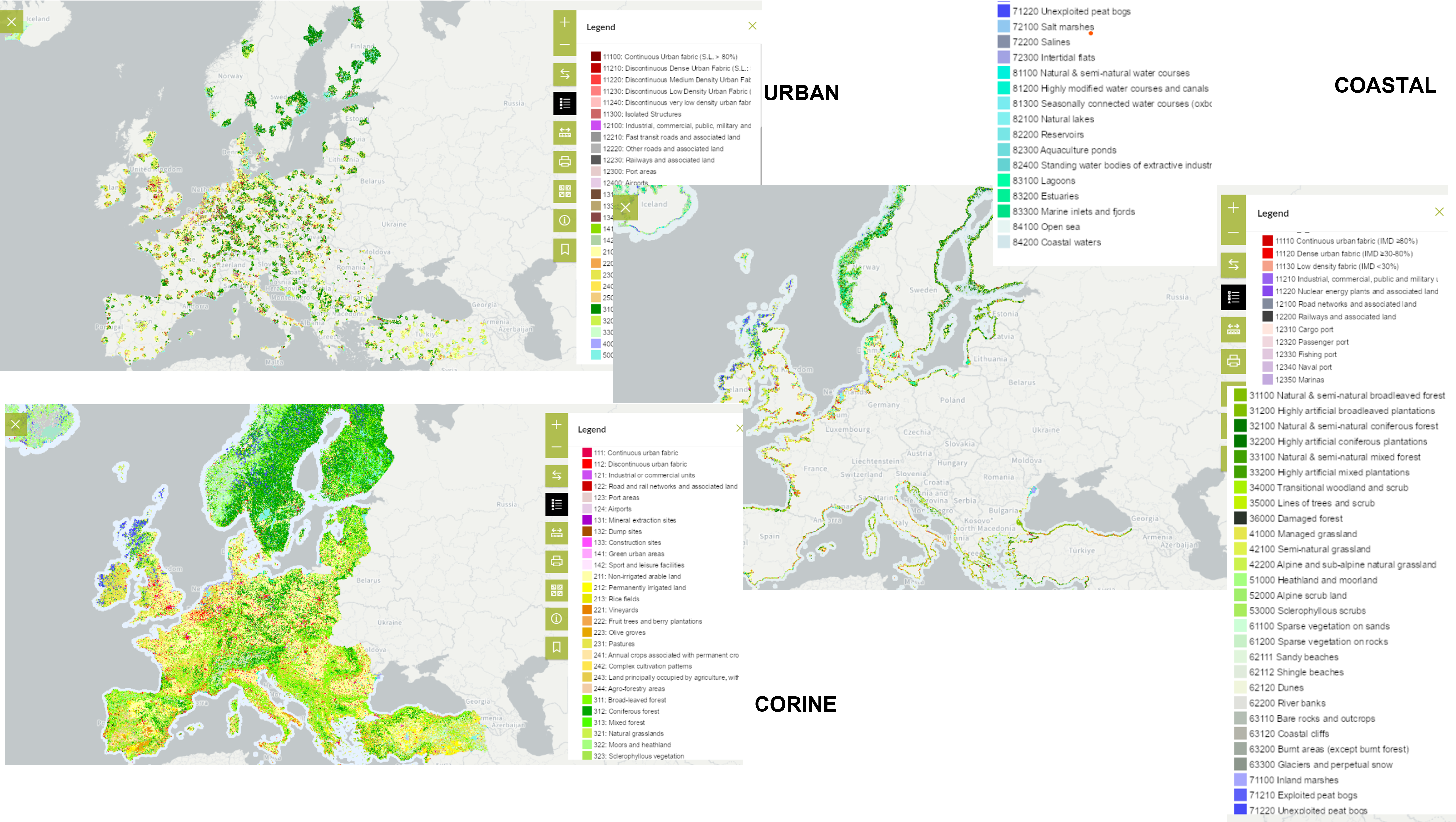
Copernicus provides comprehensive datasets on land use at various scales and resolutions. These datasets are crucial for understanding spatial heterogeneity and characterizing landscape types. In this section, we focus on three primary datasets widely used for land use classification:
1. Urban Atlas
The Urban Atlas provides detailed land use data for Functional Urban Areas (FUAs) across Europe. This dataset is particularly useful for urban studies and planning. Although its spatial coverage is limited to urban zones, its high resolution (0.25 ha for urban and 1 ha for rural areas) makes it a preferred choice for fine-scale urban analyses.
- Dataset description: Urban Atlas Overview
- Download link: Urban Atlas Data Access
The Urban Atlas 2018 dataset provides high-resolution land use and land cover data with population estimates for 788 Functional Urban Areas (FUAs) across Europe. It is ideal for urban planning and environmental assessments.
2. CORINE Land Cover (CLC)
Covering rural and urban areas, the CORINE dataset provides pan-European coverage with thematic detail spanning 44 land cover classes. This dataset is updated every six years and supports large-scale landscape analyses. While its resolution is coarser than Urban Atlas, CORINE excels in thematic coverage and integration of rural areas.
- Dataset description: CORINE Land Cover Overview
- Download link: CORINE Land Cover Data Access
The CORINE Land Cover dataset provides a Europe-wide classification at 100m resolution. While useful for regional analysis, finer-scale studies may require high-resolution local datasets.
3. Coastal Zones
The Coastal Zones dataset focuses on detailed spatial coverage of coastal areas, which is essential for addressing coastal management and conservation needs. With a high resolution of 0.5 ha, this dataset supports precise delineation of coastal features and processes.
- Dataset description: Coastal Zones Overview
- Download link: Coastal Zones Data Access
The Coastal Land Use dataset is limited to a 10km inland buffer along the coastline. If your study area extends beyond this range, consider using other datasets that cover a broader region.
Comparison of Datasets
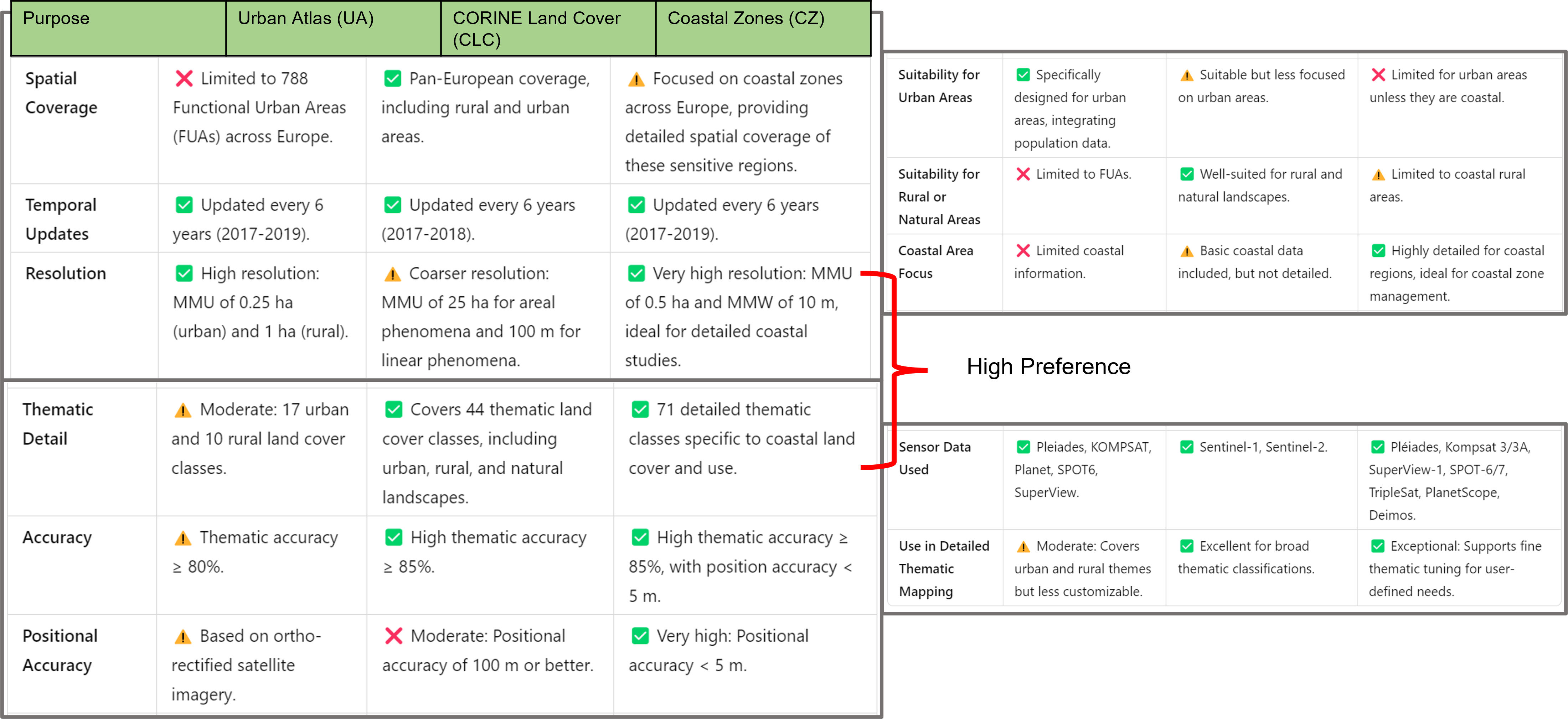
The table below provides a human-readable comparative overview of the three datasets:
| Characteristic | Urban Atlas | CORINE Land Cover | Coastal Zones |
|---|---|---|---|
| Spatial Coverage | Limited to FUAs | Pan-European | Focused on coastal areas |
| Resolution | High (0.25 ha urban, 1 ha rural) | Moderate (25 ha for areal phenomena) | High (0.5 ha) |
| Thematic Detail | 17 urban and 10 rural classes | 44 thematic classes | 71 detailed classes |
| Application | Urban planning | Broad landscape characterization | Coastal zone management |
This table compares Urban Atlas, CORINE Land Cover, and Coastal Zones based on coverage, resolution, thematic detail, and application.
The Urban Atlas focuses on functional urban areas, CORINE provides broader land cover classifications, and Coastal Land Use highlights coastal zone features.
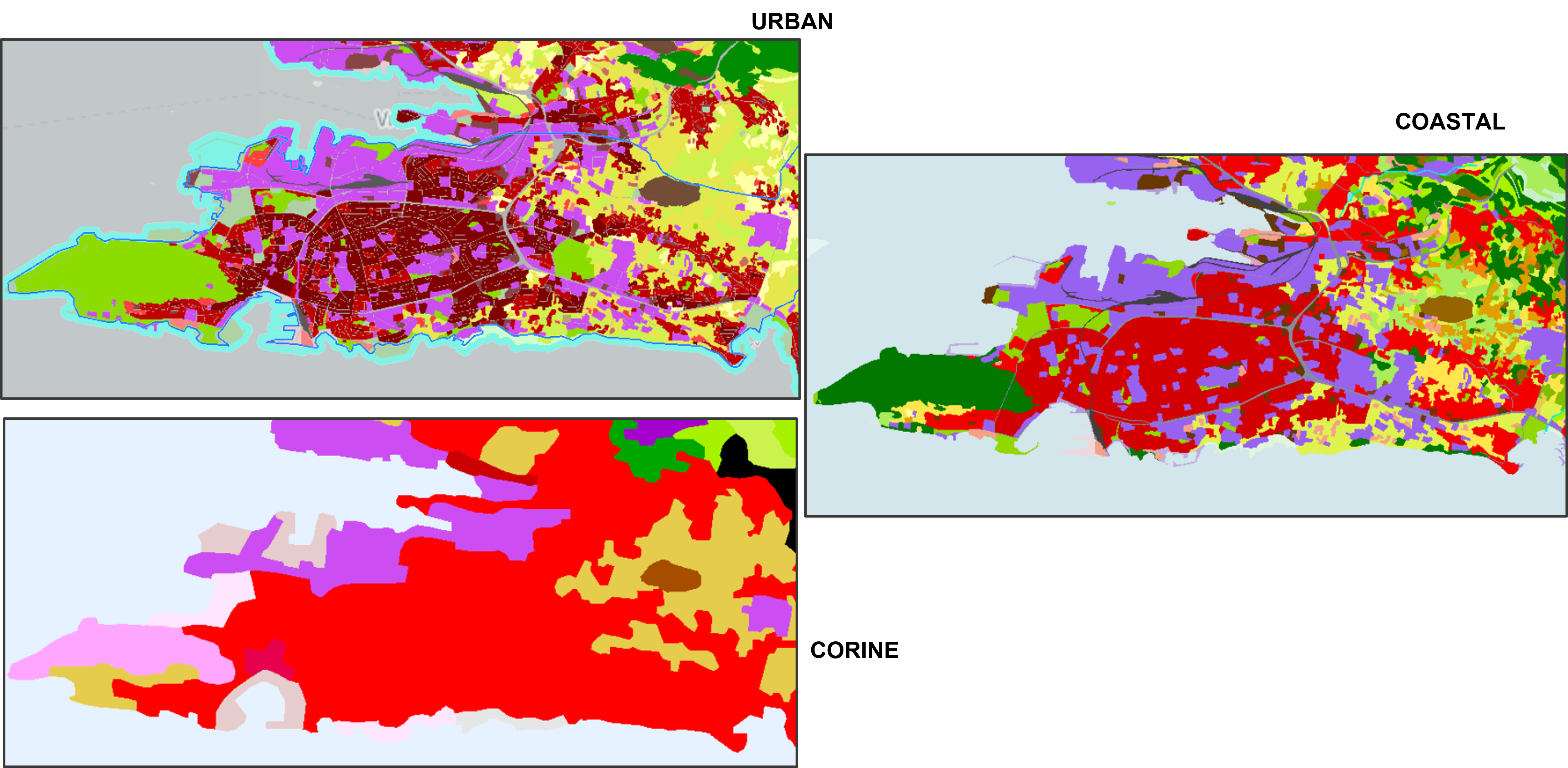
The Coastal dataset shows more artifacts, while the CORINE data lacks some level of detail, which are not very valid for change analysis because of their associated errors and uncertainties. The CORINE layers of changes (CHA) remove a lot of these issues.
Based on the needs of this workflow, the Coastal Zones dataset will be used for further analyses due to its high resolution and relevance to coastal landscapes.
Step-by-Step Download and Processing
The following steps outline the process to download, inspect, and integrate the Coastal Zones dataset into the workflow:
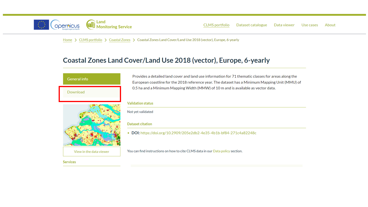
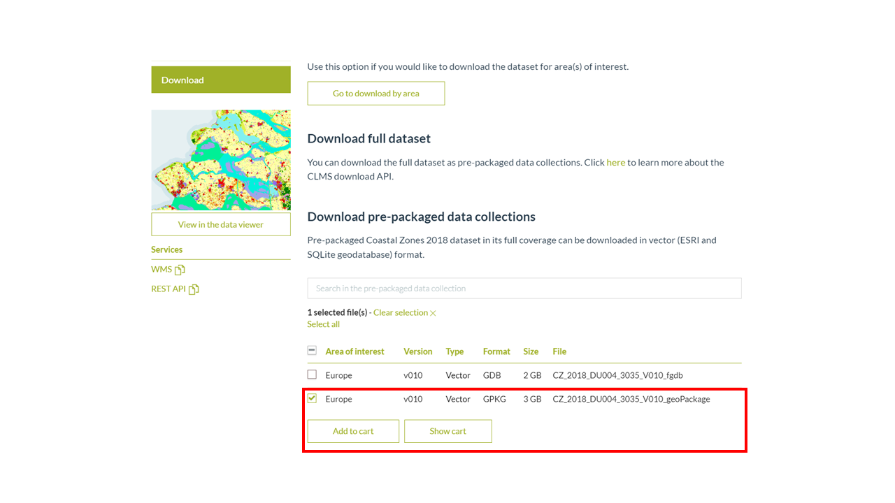
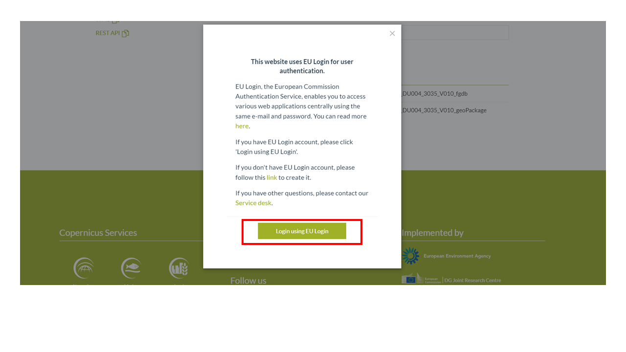
Step 1: Visit the Copernicus Land use/cover Data Portal
Access the Coastal Zones dataset by visiting the Copernicus Coastal Zones Portal. Navigate to the data access section and select the relevant dataset.
Step 2: Select and Download the Dataset
Choose the required dataset based on the region and time period of interest. Follow the download instructions provided on the portal.
Step 3: Unzip and Inspect the Data
- After downloading, unzip the dataset.
- The dataset comes in different formats:
- GPKG file – for spatial data
- QML file – for visualization
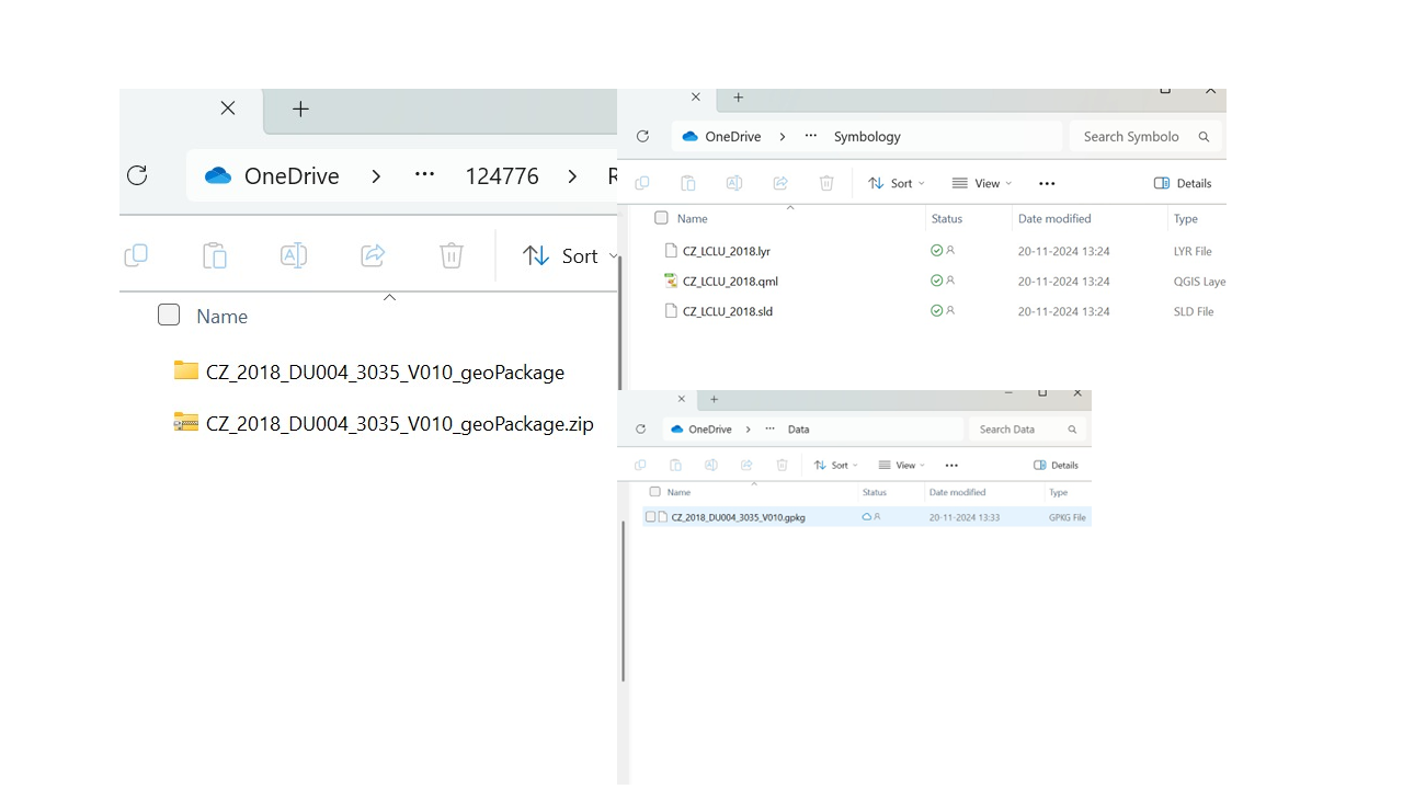
Unzip the files and inspect it contents.
- Add the GPKG file in QGIS or any preferred Desktop GIS (we will use QGIS here).
- Inspect the spatial coverage and attributes.
- Note that the dataset contains a significantly large number of shapes (>400,000).
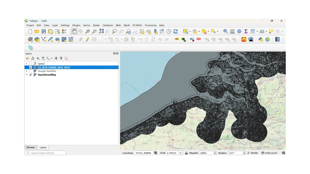
Add the layer to the map.
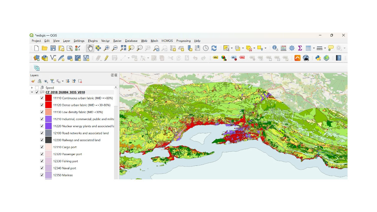
- Once loaded, add the QML file to visualize and inspect various functional units.
- Before adding the QML file, zoom into your area of interest for better clarity.
- We will not cover how to add the QML file to visualise a layer in QGIS.
- For a hands-on guide on how to do it, watch this video.
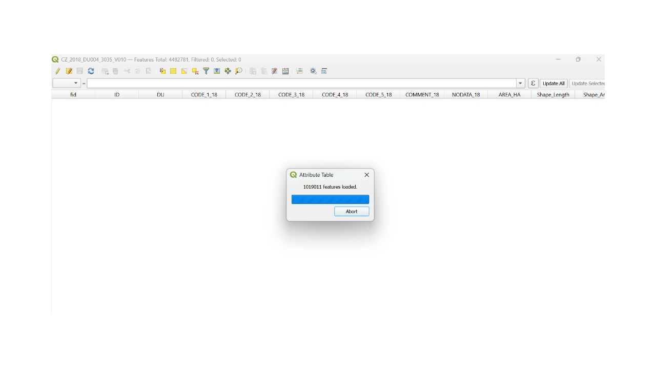
This can take a few minutes depending on your porcessor due to the file size.
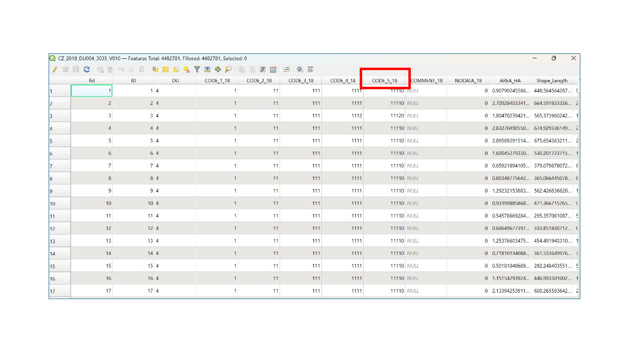
You can inspect the attributes of the dataset and take note of the columns available. For our Earth Engine processing, we will use the CODE_5_18 column, as it contains the class values for the various land use categories.
If you follow the instruction in the video, you can add the qml file which contain the colors of the land use. You will notice that the land use/cover doesnt go beyond 10km from the coast.
Step 4: Preprocess for Earth Engine
To do this in GEE,we will have to convert the dataset into a format compatible with Google Earth Engine (GEE), such as GeoTIFF or shapfiles. Use QGIS or a similar GIS tool for this step. Because the land use GPKG file contains a large number of shapes, which can make it cumbersome to work with in desktop software like ArcGIS, transitioning to a cloud computing platform like GEE is beneficial. These days, cloud platforms provide unparalleled processing power, scalability, and accessibility for handling large geospatial datasets, making them ideal for projects like this. GEE does not directly support GPKG files. Therefore, we need to export the data from GPKG into shapefiles, which are accepted by GEE. Shapefiles are more lightweight and manageable for this transition.
Step 5: Upload to Google Earth Engine
Log in to your Google Earth Engine (GEE) account and prepare to upload the preprocessed dataset. Learn how to open an Earth Engine account if you dont have. Due to the large size and complexity of the dataset, especially when working with GPKG files containing a high number of shapes (e.g., >400,000), the geometry must be simplified and split to enhance performance. GEE imposes a limit on vertices for each feature, so splitting the geometry ensures that the upload is successful and the data renders efficiently. For this step, export your dataset from GPKG to Shapefile format, as GEE does not currently support GPKG files directly.
To upload your dataset:
- Open the Asset Manager in the GEE Code Editor and click on the upload button (+).
- Select "Shape files" under the "Table Upload" section and navigate to your local Shapefile archive (.zip format) containing the .shp, .dbf, .shx, and .prj files.
- Specify an appropriate Asset ID and enable the "Split geometries" option under Advanced settings if the dataset contains highly detailed geometries.
- Click UPLOAD to start the process and monitor progress in the Task Manager.
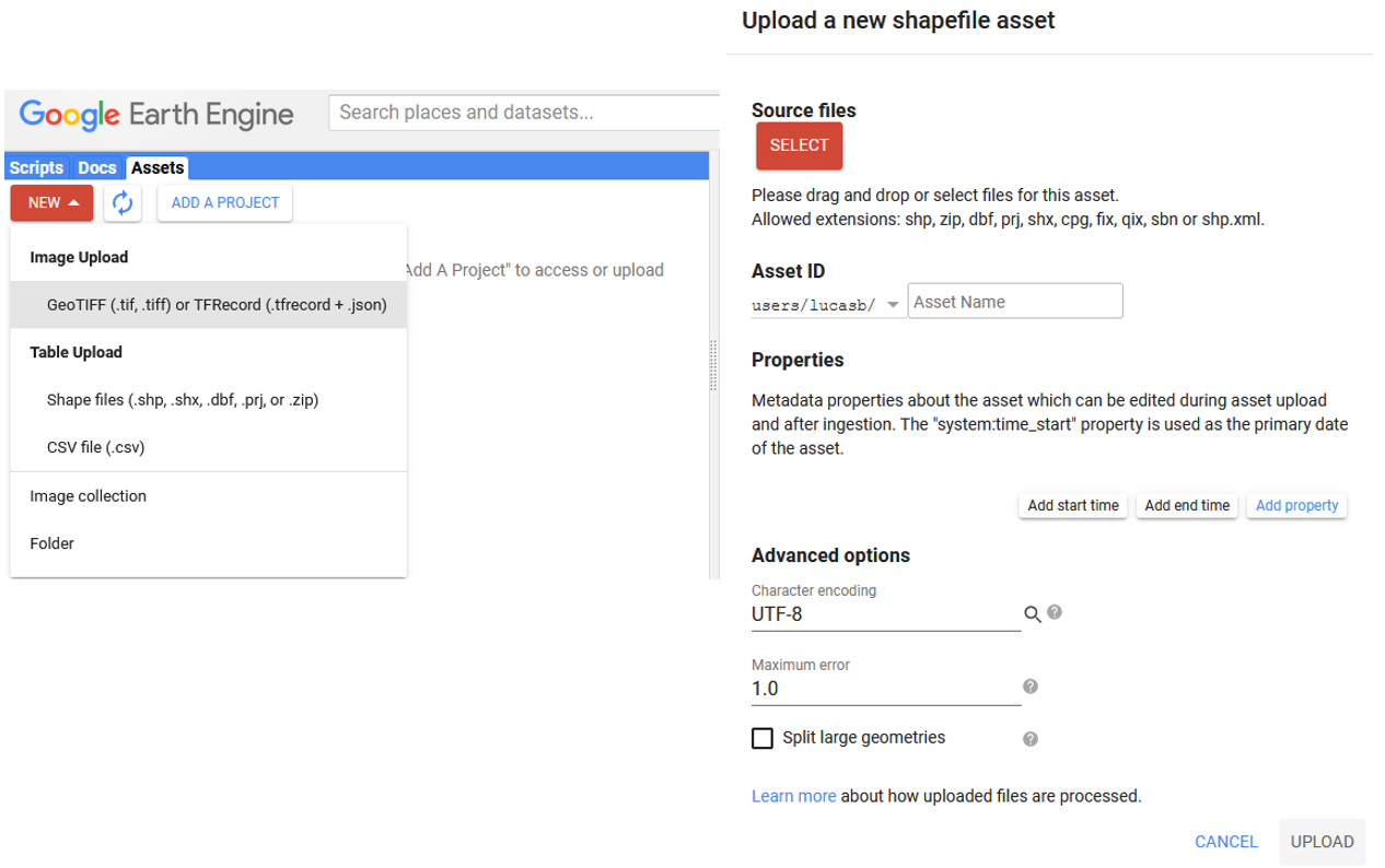
Because our vector file has more shapes than EE can handle, remember to check the 'split geometry' box.
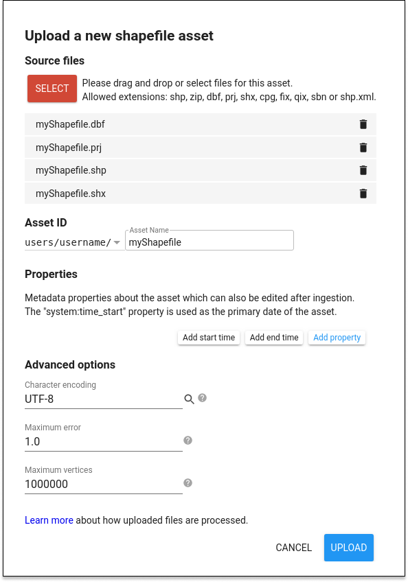
Ensure that only appropriate shapefile extensions are added. It is usually best to zip the entire folder containing the shapefiles and import it directly.
Cloud platforms like GEE provide unparalleled capabilities for processing and analyzing large geospatial datasets. These days, cloud computing is vital for handling big geospatial data because of its scalability, computational power, and ability to store and manage extensive datasets efficiently. GEE's integration with machine learning, visualization tools, and global datasets makes it an excellent choice for such workflows.
Step 6: Verify Dataset in GEE
After uploading, navigate to the Assets tab in the GEE Code Editor to ensure that the dataset appears as expected. Import the dataset into your script by copying the Asset ID and creating a FeatureCollection in your script:
// Import the uploaded dataset
var landUseDataset = ee.FeatureCollection('users/your_username/your_asset_id');

// Display the dataset on the map
Map.centerObject(landUseDataset, 10); //You can comment out this part if your browser freezes or get an error like "Collection.geometry: Geometry has too many edges (13318505 > 2000000)."
Map.addLayer(landUseDataset, {}, 'Land Use Dataset');
We can now add the layer to the map
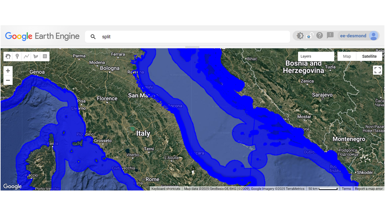
Your layer should be like this. You can also adjust the color. Note that you have not yet added the class codes. We will treat that in the next section
Land Use Dataset Creation
The creation of land use datasets is an essential step in analyzing spatial patterns and understanding land cover dynamics over time. These datasets serve as foundational inputs for various geospatial analyses, including habitat classification, urban planning, and environmental monitoring. Using Earth Engine, we can load, process, and export land use datasets efficiently while ensuring compatibility with large-scale applications.
Step 1: Load Land Use Datasets
We start by loading the land use datasets for 2012 and 2018. These datasets provide detailed land cover information for Croatia, which will be analyzed for changes over time.
// Load the asset
ar lulc2012 = ee.FeatureCollection('projects/ee-desmond/assets/lulc2012_Croatiafinal');
var lulc2018 = ee.FeatureCollection('projects/ee-desmond/assets/lulc2018_Croatiafinal');
The ee.FeatureCollection function is used to load the datasets.
Each dataset contains land use features for Croatia, which are stored in a structured format compatible with Earth Engine operations.
-->Step 2: Define the Color Palette for Land Cover Classes
To enhance visualization, we define a color palette and descriptions for each land cover class. This ensures that each class is visually distinct and easy to interpret.
// Define the color palette for each land use class
  var landCoverClasses = {
    11110: {color: '#d20000', description: 'Continuous urban fabric (IMD >= 80%)'},
    11120: {color: '#f20000', description: 'Dense urban fabric (IMD >= 30-80%)'},
    11130: {color: '#f5a18a', description: 'Low density fabric (IMD < 30%)'},
    11210: {color: '#9862f0', description: 'Industrial, commercial, public, and military units'},
    11220: {color: '#8748ee', description: 'Nuclear energy plants and associated land'},
    12100: {color: '#838b9d', description: 'Road networks and associated land'},
    12200: {color: '#404040', description: 'Railways and associated land'},
    12310: {color: '#ffe6de', description: 'Cargo port'},
    12320: {color: '#f0d7de', description: 'Passenger port'},
    12330: {color: '#FF1493', description: 'Fishing port'},
    12340: {color: '#800000', description: 'Naval port'},
    12350: {color: '#DB7093', description: 'Marinas'},
    12360: {color: '#9932CC', description: 'Local multi-functional harbours'},
    12370: {color: '#8B008B', description: 'Shipyards'},
    12400: {color: '#4B0082', description: 'Airports and associated land'},
    13110: {color: '#966401', description: 'Mineral extraction sites'},
    13120: {color: '#A52A2A', description: 'Dump sites'},
    13130: {color: '#B8860B', description: 'Construction sites'},
    13200: {color: '#D2691E', description: 'Land without current use'},
    14000: {color: '#91d700', description: 'Green urban, sports, and leisure facilities'},
    21100: {color: '#ffffa8', description: 'Arable irrigated and non-irrigated land'},
    21200: {color: '#b9c151', description: 'Greenhouses'},
    22100: {color: '#f3830b', description: 'Vineyards, fruit trees, and berry plantations'},
    22200: {color: '#df9f00', description: 'Olive groves'},
    23100: {color: '#ffe6a6', description: 'Annual crops associated with permanent crops'},
    23200: {color: '#ffe64d', description: 'Complex cultivation patterns'},
    23300: {color: '#e6cc4d', description: 'Land principally occupied by agriculture'},
    23400: {color: '#edc69f', description: 'Agro-forestry'},
    31100: {color: '#82be00', description: 'Natural & semi-natural broadleaved forest'},
    31200: {color: '#82be00', description: 'Highly artificial broadleaved plantations'},
    32100: {color: '#008000', description: 'Natural & semi-natural coniferous forest'},
    32200: {color: '#027800', description: 'Highly artificial coniferous plantations'},
    33100: {color: '#41a000', description: 'Natural & semi-natural mixed forest'},
    33200: {color: '#556B2F', description: 'Highly artificial mixed plantations'},
    34000: {color: '#a9f100', description: 'Transitional woodland and scrub'},
    35000: {color: '#8B0000', description: 'Lines of trees and scrub'},
    36000: {color: '#A0522D', description: 'Damaged forest'},
    41000: {color: '#BDB76B', description: 'Managed grassland'},
    42100: {color: '#DAA520', description: 'Semi-natural grassland'},
    42200: {color: '#F4A460', description: 'Alpine and sub-alpine natural grassland'},
    51000: {color: '#8B4513', description: 'Heathland and moorland'},
    52000: {color: '#DEB887', description: 'Alpine scrub land'},
    53000: {color: '#FFDAB9', description: 'Sclerophyllous scrubs'},
    61100: {color: '#D2B48C', description: 'Sparse vegetation on sands'},
    61200: {color: '#F5DEB3', description: 'Sparse vegetation on rocks'},
    62111: {color: '#FFE4C4', description: 'Sandy beaches'},
    62112: {color: '#FFA07A', description: 'Shingle beaches'},
    62120: {color: '#FFD700', description: 'Dunes'},
    62200: {color: '#FFEBCD', description: 'River banks'},
    63110: {color: '#FAF0E6', description: 'Bare rocks and outcrops'},
    63120: {color: '#F0E68C', description: 'Coastal cliffs'},
    63200: {color: '#D3D3D3', description: 'Burnt areas (except burnt forest)'},
    63300: {color: '#C0C0C0', description: 'Glaciers and perpetual snow'},
    71100: {color: '#B0E0E6', description: 'Inland marshes'},
    71210: {color: '#ADD8E6', description: 'Exploited peat bogs'},
    71220: {color: '#464af8', description: 'Unexploited peat bogs'},
    72100: {color: '#91c8f0', description: 'Salt marshes'},
    72200: {color: '#858fa7', description: 'Salines'},
    72300: {color: '#a2a3e3', description: 'Intertidal flats'},
    81100: {color: '#00f1dd', description: 'Natural & semi-natural water courses'},
    81200: {color: '#00f4cf', description: 'Highly modified water courses and canals'},
    81300: {color: '#79ecf0', description: 'Seasonally connected water courses'},
    82100: {color: '#82f0f0', description: 'Natural lakes'},
    82200: {color: '#78e6e6', description: 'Reservoirs'},
    82300: {color: '#6edcdc', description: 'Aquaculture ponds'},
    82400: {color: '#64d2d2', description: 'Standing water bodies of extractive industrial sites'},
    83100: {color: '#00ffa6', description: 'Lagoons'},
    83200: {color: '#00f096', description: 'Estuaries'},
    83300: {color: '#00e187', description: 'Marine inlets and fjords'},
    84100: {color: '#e6f5f3', description: 'Open sea'},
    84200: {color: '#d2e6eb', description: 'Coastal waters'}
  };
The landCoverClasses object maps class codes to their respective colors and descriptions. These properties are later used for styling the dataset in Earth Engine.
Step 3: Define Croatia Coastal Boundaries
We focus the analysis on Croatia's coastal region by defining a geographic boundary. This ensures that only relevant features are included in the dataset.
// Define Croatia's coastal bounds
var croatiaCoastalBounds = ee.Geometry.Polygon([
  [13.5, 44.0], [18.5, 44.0], [18.5, 42.0], [13.5, 42.0], [13.5, 44.0]
]);
A polygon geometry is created to delineate the coastal region of Croatia. The filterBounds function will use this boundary to extract relevant features from the datasets.
Step 4: Filter the Dataset to the Coastal Region
The land use datasets are filtered to include only features within the coastal boundaries. This reduces computational overhead and focuses the analysis on the area of interest.
// Filter datasets for 2012 and 2018 to the coastal region
var coastalLulc2012 = lulc2012.filterBounds(croatiaCoastalBounds);
var coastalLulc2018 = lulc2018.filterBounds(croatiaCoastalBounds);
The filterBounds method is used to extract features that intersect the defined coastal region. This step ensures that only relevant data is included in subsequent analyses.
Step 5: Rasterize the Dataset
We convert the feature collections into raster images, which are more suitable for pixel-based analyses and visualizations.
// Rasterize the 2012 dataset
var rasterized2012 = coastalLulc2012.map(function(feature) {
  var code = feature.get('CODE_5_12'); // Use the field for the 2012 dataset
  return feature.set('class', code); // Set the class based on CODE_5_12
}).reduceToImage(['class'], ee.Reducer.first());

// Rasterize the 2018 dataset
var rasterized2018 = coastalLulc2018.map(function(feature) {
  var code = feature.get('CODE_5_18'); // Use the field for the 2018 dataset
  return feature.set('class', code); // Set the class based on CODE_5_18
}).reduceToImage(['class'], ee.Reducer.first());
The reduceToImage function is used to generate raster images from the feature collections. Each pixel in the raster represents a land use class, with values corresponding to the class property.
Step 6: Style and Visualize the Rasterized Datasets
We apply the color palette to the rasterized datasets and visualize them on the map for inspection.
// Extract the color palette from landCoverClasses
var palette = Object.keys(landCoverClasses).map(function(key) {
  return landCoverClasses[key].color; // Ensure only colors are extracted
});

// Add the rasterized 2012 layer to the map
Map.addLayer(rasterized2012, {min: 11110, max: 84200, palette: palette}, 'Coastal Land Use 2012');

// Add the rasterized 2018 layer to the map
Map.addLayer(rasterized2018, {min: 11110, max: 84200, palette: palette}, 'Coastal Land Use 2018');
The color palette ensures that each class is visually distinct, making it easier to interpret the rasterized datasets. Adding the layers to the map allows for visual inspection and verification.
Step 7: Add a Legend for Visualization
To enhance interpretability, we create a legend that displays the color and description for each land use class.
// Create the legend container
var legend = ui.Panel({
  style: {
    position: 'bottom-left',
    padding: '0px',
    backgroundColor: '#f0f0f0'
  }
});

// Add a checkbox to toggle the legend visibility
var showLegend = ui.Checkbox({
  label: 'Show Legend',
  value: true,  // Initially checked to show the legend
  style: {
    fontSize: '10px',
    padding: '0px',
    backgroundColor: '#f0f0f0'
  }
});
legend.add(showLegend);

// Create columns for the legend items
var column1 = ui.Panel({
  style: {
    padding: '5px',
    backgroundColor: '#f0f0f0'
  }
});

// Container panel to hold all columns
var columns = ui.Panel({
  layout: ui.Panel.Layout.Flow('horizontal'),
  style: {
    backgroundColor: '#f0f0f0'
  }
});
columns.add(column1);

// Helper function to create a legend row
var makeRow = function(color, description) {
  var colorBox = ui.Label({
    style: {
      backgroundColor: color,
      padding: '4px',
      margin: '0 4px 4px 0'
    }
  });
  var label = ui.Label({
    value: description,
    style: {
      margin: '0 0 4px 6px',
      fontSize: '10px',
      backgroundColor: '#f0f0f0'
    }
  });
  return ui.Panel({
    widgets: [colorBox, label],
    layout: ui.Panel.Layout.Flow('horizontal'),
    style: {
      backgroundColor: '#f0f0f0'
    }
  });
};

// Populate the legend
Object.keys(landCoverClasses).forEach(function(key) {
  var color = landCoverClasses[key].color;
  var description = landCoverClasses[key].description;
  column1.add(makeRow(color, description));
});

// Add the legend to the map
legend.add(columns);
Map.add(legend);
The legend provides a visual reference for interpreting the land use classes, making the map more user-friendly and informative.
Step 8: Export the Rasterized Datasets
Finally, we export the rasterized datasets as assets for further analysis or sharing.
// Export rasterized 2012 dataset
Export.image.toAsset({
  image: rasterized2012,
  description: 'Coastal_Land_Use_2012',
  assetId: 'projects/ee-desmond/assets/Coastal_Land_Use_2012',
  region: croatiaCoastalBounds,
  scale: 30,
  crs: 'EPSG:4326',
  maxPixels: 1e13
});

// Export rasterized 2018 dataset
Export.image.toAsset({
  image: rasterized2018,
  description: 'Coastal_Land_Use_2018',
  assetId: 'projects/ee-desmond/assets/Coastal_Land_Use_2018',
  region: croatiaCoastalBounds,
  scale: 30,
  crs: 'EPSG:4326',
  maxPixels: 1e13
});
Exporting the datasets ensures that they are available for future analyses or integration into other workflows. The Export.image.toAsset function saves the data as assets within the Earth Engine environment.
Our Land use/cover data is ready for further analysis in Google Earth Engine. We will use this data as the functional unit and the basis for vreating other datasets like EUNIS, landscape Archetypes, Ecosystem service Map and risk exposures
Landscape Characterisation
Understanding landscape archetypes is a critical step in spatial analysis, providing insights into how different land use and land cover classes interact across a given region. The concept of landscape archetypes integrates bio-physical, socio-economic, and governance layers to create meaningful spatial patterns that aid in decision-making for environmental planning, impact assessments, and conservation strategies.
In this guide, we will develop a classification scheme for landscape archetypes i.e bio-physical using the land use dataset we created earlier. The workflow includes loading datasets, defining classifications, applying a reclassification technique, and visualizing the results. The classification process is based on CORINE land cover data, which serves as the basis for defining unique landscape archetypes according to their spatial patterns.
Bio-physical Domain
Step 1: Load Land Use Data
The first step involves loading the land use datasets for 2012 and 2018. These datasets will serve as the basis for reclassifying landscape archetypes.
// Load the asset
var lulc2012 = ee.FeatureCollection('projects/ee-desmond/assets/lulc2012_Croatiafinal');
var lulc2018 = ee.FeatureCollection('projects/ee-desmond/assets/lulc2018_Croatiafinal');
The ee.FeatureCollection function is used to load the vector datasets containing land use classifications for Croatia in 2012 and 2018. Each dataset consists of multiple features representing distinct land cover classes.
Step 2: Define Croatia’s Coastal Boundaries
To limit our analysis to the coastal region of Croatia, we define a geographic boundary using a polygon geometry.
// Define Croatia's coastal bounds
var croatiaCoastalBounds = ee.Geometry.Polygon([
  [13.5, 44.0], [18.5, 44.0], [18.5, 42.0], [13.5, 42.0], [13.5, 44.0]
]);
The ee.Geometry.Polygon function creates a polygon that defines the spatial extent of the study area. This boundary is later used to filter the dataset and extract only the relevant features.
Step 3: Filter the Dataset to the Coastal Region
Once the study boundary is established, we filter the dataset to retain only the features that fall within this region.
// Filter the datasets to Croatia's coastal region
var coastalLulc2012 = lulc2012.filterBounds(croatiaCoastalBounds);
var coastalLulc2018 = lulc2018.filterBounds(croatiaCoastalBounds);
The filterBounds method is applied to extract only those features that intersect with the defined polygon, ensuring that our analysis focuses solely on Croatia’s coastal areas.
Step 4: Define Landscape Archetypes
We define a classification scheme that groups land cover classes into broader landscape archetypes based on their ecological and functional similarities.
// Define landscape archetypes
  var landscapeArchetypes = {
    '1': { classes: ['11110', '11120', '11130', '11210', '11220', '12100', '12200'], color: '#636363', description: 'Urban' },
    '2': { classes: ['12310', '12320', '12330', '12340', '12350', '12360', '12370', '12400'], color: '#969696', description: 'Coastal Urban' },
    '3': { classes: ['13110', '13120', '13130', '13200'], color: '#cccccc', description: 'Industrial' },
    '4': { classes: ['14000'], color: '#91d700', description: 'Recreational & Leisure Areas' },
    '5': { classes: ['21100', '21200', '23300', '23400'], color: '#91d700', description: 'Rural (Riparian Zone, Floodplain, Interfluvium Flat Areas)' },
    '6': { classes: ['23100', '23200', '22200', '22100'], color: '#df9f00', description: 'Rural (Hillside, Interfluvium Hilly Areas)' },
    '7': { classes: ['31100', '31200', '31300', '32100', '32200', '33100', '33200', '34000'], color: '#80ff00', description: 'Forested' },
    '8': { classes: ['35000', '36000', '41000', '42100'], color: '#a63603', description: 'Mountainous (Hillside, Hollow/Torrent)' },
    '9': { classes: ['42200', '51000', '52000', '53000', '61100'], color: '#78c679', description: 'Rural' },
    '10': { classes: ['62111', '62112', '62120', '61100'], color: '#ffcc99', description: 'Coastal (Beach-Dune System, Coastal Land-Claim Areas)' },
    '11': { classes: ['62200', '63120', '63200'], color: '#7fff00', description: 'Coastal Rural (Estuary, Polder)' },
    '12': { classes: ['71100', '71210', '71220', '72100', '72200', '72300', '63300'], color: '#a6e6ff', description: 'Wetlands & Marshes' },
    '13': { classes: ['81100', '81200', '81300', '82100', '82200', '82300', '82400'], color: '#4da6ff', description: 'Inland Water Bodies' },
    '14': { classes: ['83100', '83200', '83300', '84100', '84200'], color: '#00bfff', description: 'Marine (Subtidal Coast)' }
};
The landscapeArchetypes object maps groups of land cover codes to their corresponding archetypes. Each archetype is associated with a unique color and description to facilitate interpretation.
Step 5: Remap Land Cover Classes
To convert the original land cover classifications into archetypes, we create a mapping function that translates each class into its corresponding archetype.
// Prepare lists for remapping
var fromList = [];
var toList = [];
var palette = [];
var descriptions = [];

Object.keys(landscapeArchetypes).forEach(function(archetypeId) {
  var archetype = landscapeArchetypes[archetypeId];
  var archetypeIdInt = parseInt(archetypeId);
  archetype.classes.forEach(function(classCode) {
    fromList.push(parseInt(classCode));
    toList.push(archetypeIdInt);
  });
  palette.push(archetype.color);
  descriptions.push(archetype.description);
});
The remap function is used to convert the original land cover class values into landscape archetypes by replacing each class with its respective archetype ID. This step ensures that each pixel is assigned a meaningful category that aligns with the predefined archetype classification.
Step 6: Apply Reclassification
This step involves reclassifying the 2012 and 2018 datasets based on the remapping criteria.
// Reclassify the datasets
var codeImage2012 = coastalLulc2012.reduceToImage(['CODE_5_12'], ee.Reducer.first()).rename('code2012');
var codeImage2018 = coastalLulc2018.reduceToImage(['CODE_5_18'], ee.Reducer.first()).rename('code2018');

var archetypeImage2012 = codeImage2012.remap(fromList, toList).rename('archetype2012');
var archetypeImage2018 = codeImage2018.remap(fromList, toList).rename('archetype2018');
Here you will realise we use 'CODE_5_12' and CODE_5_18' as columns to remap, this is because both datasets contains the class ids or class values to the land use. The reduceToImage function converts the vector dataset into a raster, while remap assigns each pixel a new value based on the archetype classification.
Step 7: Apply Reclassification and visualise
  // Mask out any pixels not in the 'toList' (i.e., archetypes)
  archetypeImage2012 = archetypeImage2012.updateMask(archetypeImage2012.neq(0));
  archetypeImage2018 = archetypeImage2018.updateMask(archetypeImage2018.neq(0));

  // Add the reclassified raster layers to the map
  Map.addLayer(archetypeImage2012.clip(croatiaCoastalBounds), {min: 1, max: 14, palette: palette}, 'Reclassified Landscape Archetypes 2012');
  Map.addLayer(archetypeImage2018.clip(croatiaCoastalBounds), {min: 1, max: 14, palette: palette}, 'Reclassified Landscape Archetypes 2018');

  // Center the map on Croatia's coastal region
  Map.centerObject(croatiaCoastalBounds, 12);

  // Create the legend container
  var legend = ui.Panel({
    style: {
      position: 'bottom-left',
      padding: '8px',
      backgroundColor: '#f0f0f0'
    }
  });

  legend.add(ui.Label({
    value: 'Landscape Archetypes',
    style: {fontWeight: 'bold', fontSize: '14px', margin: '0 0 8px 0'}
  }));

  for (var i = 0; i < descriptions.length; i++) {
    var colorBox = ui.Label({
      style: {
        backgroundColor: palette[i],
        padding: '8px',
        margin: '0 8px 8px 0'
      }
    });
    var label = ui.Label({
      value: descriptions[i],
      style: {margin: '0 0 8px 0'}
    });
    legend.add(ui.Panel({
      widgets: [colorBox, label],
      layout: ui.Panel.Layout.Flow('horizontal')
    }));
  }

  // Add the legend to the map
  Map.add(legend);
  Map.setCenter(16.3521, 43.5384, 12);
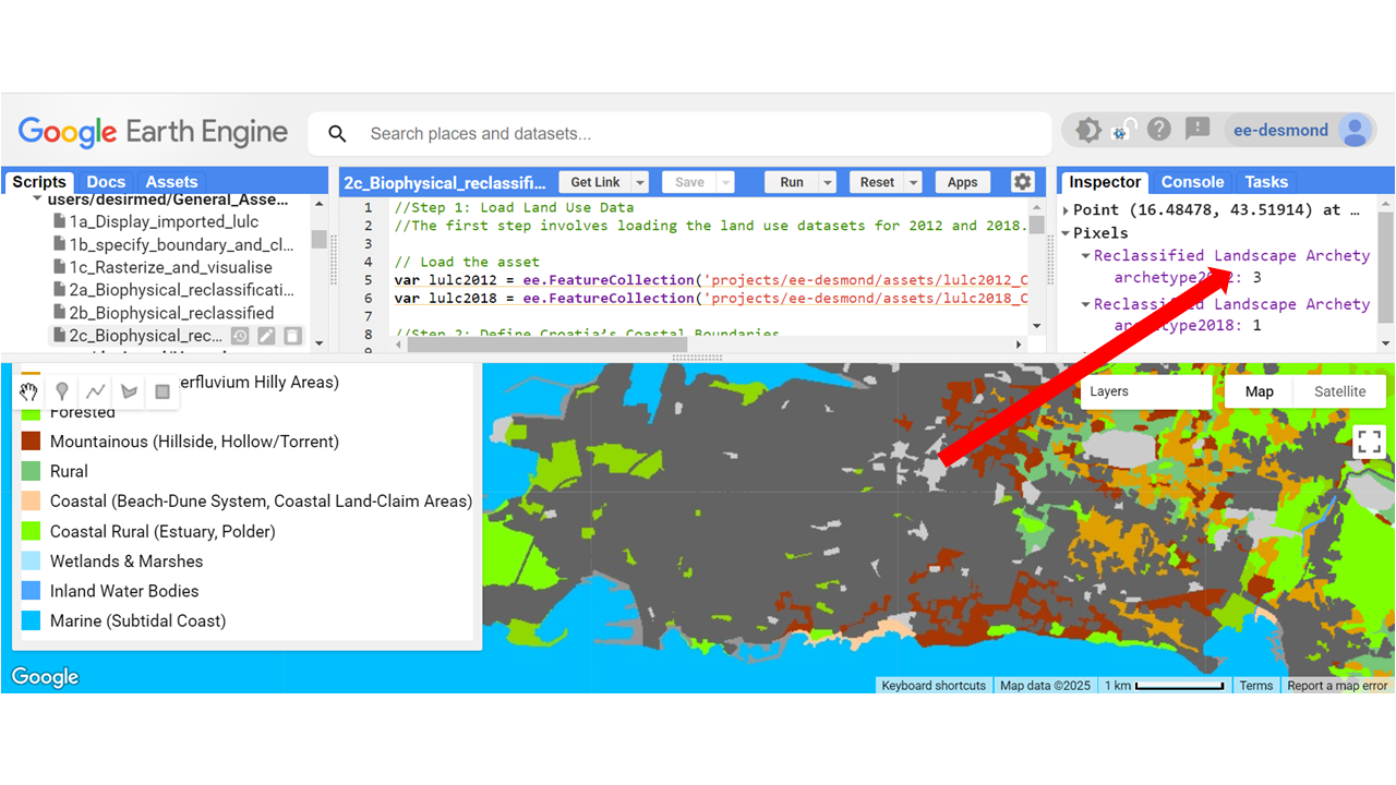
You can inspect a pixel and try to understand the result by corresponding the values to their respective legen class names You can toggle betweeen both years to see which archetypes are changing from what. An example of this in your image.
Technical Process Overview
- Data Preparation: The input datasets consist of land use classifications derived from CORINE data (2012 and 2018). Each land cover class is assigned a unique integer code.
- Reclassification Using
remap(): Theremap()function is applied to translate CORINE land cover classes into predefined archetypes. Each archetype groups multiple land cover classes based on shared ecological and functional characteristics. - Binary Masking with
eq()andor(): Pixel values are conditionally filtered to match the target landscape archetypes, ensuring that only relevant land cover types are included. - Rule-Based Aggregation: Similar land cover types (e.g., forests, agricultural lands) are grouped under broader landscape units to enhance interpretability and spatial generalization.
- Vectorization and Area Computation: Raster data is converted into vector polygons, and each feature is assigned an area measurement to enable statistical assessments.
- Visualization and Legend Creation: The reclassified maps are visualized using a predefined color palette, and a legend is dynamically generated to improve user interpretation.
- Exporting Outputs: The final archetype datasets are exported to Google Earth Engine assets and Google Drive for further analysis and external use.
Potential Issues and Considerations
- Loss of Granular Detail: Aggregating land cover classes into broad archetypes can obscure finer ecological variations (e.g., differentiating between mixed forests and coniferous forests).
- Potential Misclassification: The binary classification approach using
eq()andor()can lead to misclassification if a land cover pixel aligns with multiple archetypes (Panpan et al., 2024). - Landscape Artifacts and Temporal Mismatches: The underlying land cover dataset is based on 2018 data, meaning that landscape changes in the past six years are not reflected in the current classification (Sousa et al., 2020).
References
- Panpan et al., 2024 - Comparative validation of recent 10 m-resolution global land cover maps.
- Sousa et al., 2020 - Reconstructing Three Decades of Land Use and Land Cover.
For interactive visualization, explore the generated maps on Landscapearchetypes-biophysical.
Other Datasets
Following the Biophysical landscapes, we will explore additional datasets such as EUNIS, Points of Interest (POI), population, river basins, hydrosheds, and flood probability data. Similar detailed steps will be provided to guide you through the download, preprocessing, and integration of these datasets.
Socio-Economic
Understanding landscapes extends beyond ecological and physical characteristics; socio-economic factors play a crucial role in how landscapes function. Socio-economic landscape characterization refers to analyzing human activities, economic infrastructures, and demographics to assess their influence on land use, biodiversity, and resilience.
Recent studies emphasize that integrating socio-economic data with landscape ecological analysis enhances decision-making for Nature-Based Solutions (NBS) and sustainable land use planning (Zhang & Lin, 2023; Khoroshev & Emelyanova, 2024).
Mapping socio-economic indicators can include and not limited to:
- Identify economic hubs and services influencing environmental pressures (Moos et al., 2022).
- Analyze human-nature interactions affecting biodiversity conservation (Morariu et al., 2023).
- Support climate adaptation strategies by assessing economic vulnerability (Edidin, 2024).
However, detailed socio-economic spatial data is often fragmented or inaccessible, limiting its integration into landscape assessments at high resolution (Cultice et al., 2023).
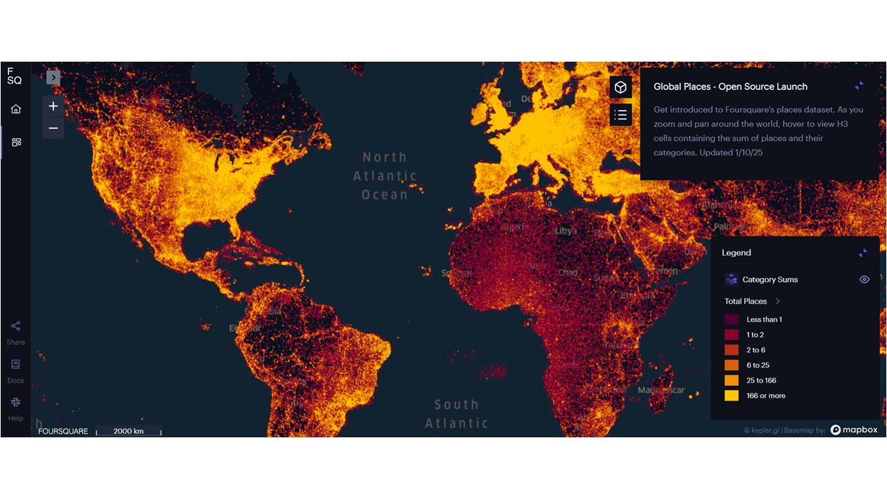
Using Foursquare’s POI Dataset for Socio-Economic indicators
Thanks to global location intelligence, we now have access to 100 million+ Points of Interest (POI) from Foursquare’s Open Source Places dataset.
Apart from for instances extracting socio-economic indicators from a land use data (which is often difficult), this is the most available dataset we can rely on. It is advisable to consult with stakeholders if these indicators align with what they will consider as receptors necessary for underdtanding their system and the assessment and support of NbS. But we will use this dataset to:
- Map economic activity and infrastructure (e.g., businesses, services, transport hubs).
- Assess functional land use and socio-economic interactions with ecological areas.
- Validate data with regional stakeholders to ensure relevance.
Dataset Overview & Limitations
The dataset includes:
- Location metadata (e.g., coordinates, place names).
- Hierarchical categorization (e.g., type of business or infrastructure).
Example JSON of a POI:
{
  "type": "Feature",
  "properties": {
    "name": "Mauricio's Manor",
    "level2_category_name": "Accommodation"
  },
  "geometry": {
    "type": "Point",
    "coordinates": [-122.440572, 37.765877]
  }
}
Challenges & Limitations
- Potential location inaccuracies (GPS shifts, outdated places).
- Incomplete rural coverage (urban bias in data collection).
- Categorization inconsistencies across different regions.
Exploring, Downloading, and Preprocessing the Data
Step 1: Accessing Foursquare’s POI Data
- We will first inspect how the POIS look like on a globe map.
- Go to Foursquare Open Source Places.
- Click on Explore and then visualise pois.

- Now you can see how the data is visualise globally. You can display this differently by toggling betwwen the visualisation parameter. It was has a 2D and 3D map view.
- Thanks to Fused, they have partitioned these points into easily accessible GeoParquet files, and hosted them on Source Cooperative. So we can easily extract this data for use.
- Go to Foursquare Open Source Places.
- Search for your region of interest.
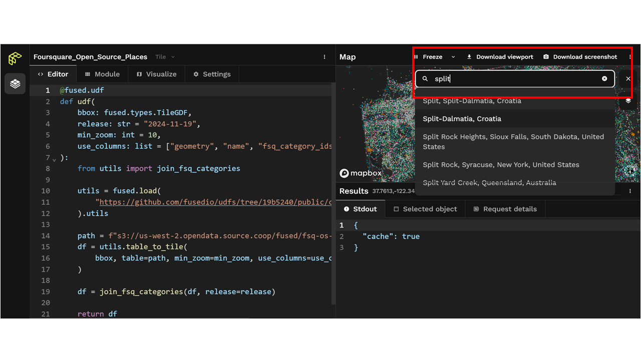
- Click on a POI to inspect its attributes.
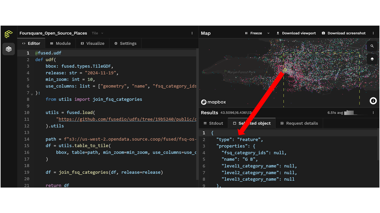
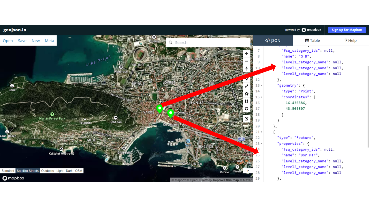
Inspecting a Point Feature in the Foursquare Dataset
After selecting a **Point of Interest (POI)** in the **Foursquare Open Source Places** interface, the feature's details will appear in **JSON format** within the console.
JSON (**JavaScript Object Notation**) is a lightweight data format used for storing and exchanging structured information. In this dataset, each POI is represented as a **GeoJSON Feature**, containing **properties** (metadata) and **geometry** (location).
Example JSON Feature:
{
  "type": "Feature",
  "properties": {
    "name": "Mauricio's Manor",
    "level2_category_name": "Accommodation"
  },
  "geometry": {
    "type": "Point",
    "coordinates": [-122.440572, 37.765877]
  }
}
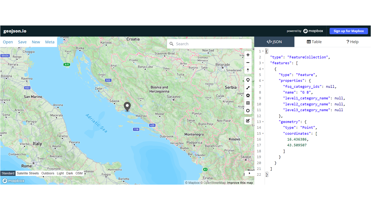
To confirm if the extracted location matches the real-world coordinates or information we need to classify this KCS:
- Copy the entire **JSON feature** from the Foursquare console.
- Go to GeoJSON.io.
- Paste the copied **JSON feature** into the **right-side text editor**.
- The **location marker** will automatically appear on the interactive map. If you have idenfitied a another socio-economic data that you will want to map, copy that and paste
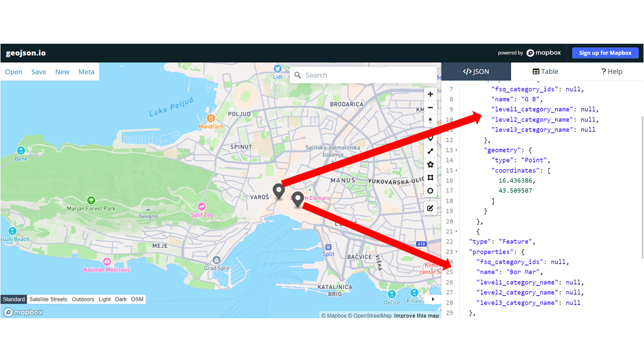
Inspecting the Point’s Accuracy
- Toggle between Satellite and Street View to check if the POI is correctly positioned.
- Compare the **category and attributes** (e.g., business name) with known data.
- If the location appears incorrect, this suggests a **possible data quality issue** (e.g., outdated coordinates).
This manual inspection helps verify **data reliability** before large-scale analysis. For instance if the social economic indicator is positioned well, it attributes are correct and if you will like to consider this as a receptor. When you are satisfied with the information you have a point, you can then export this and group them into the categories a.k.a Key Community Systems (KCS) useful for your assessment. However, since verifying thousands of points individually is impractical, we will use **spatial aggregation** in the next step to analyze and group the pattern of these KCS at a broader scale.
Understanding Aggregation in Spatial Analysis
Spatial Aggregation calculates statistics in areas where an input layer overlaps a boundary layer. You can perform a spatial aggregate on maps with two layers: one area layer with the boundaries that will be used for aggregation (for example, countries, cities, districts or community) and one layer to aggregate. We will use area layers (in this case our community boundaries) to summarize only the proportions of the point features that are within the input boundary and group them into broader categories. So for instance, Health, Education etc. This helps us to know what categories of KCS are within a certain area which can be used for other exposure/vulnerability analysis. Remember that our poi data is already in categories.
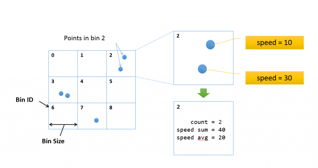
Imagine you have **100,000 individual KCS locations**. Instead of analyzing them **one by one**, you can **aggregate** them by:
- Summing up **the number(count) of KCS in categories in each neighborhood**.
- Calculating **the average socio-economic density per region**.
- Grouping data **by categories** (e.g., commercial areas vs. residential zones).
To do this lets first download the data
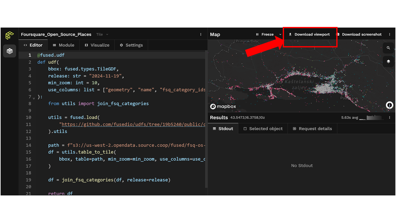
Step 2: Downloading POI Data
- Zoom into your area to capture detailed POI data.
- Click "Download Viewpoint". It automatically download all poi on map canvas in **JSON format**.
- Save the downloaded data into a folder or directory.
- The next step now will be to convert the json file into a **shapefile** to be used in Earth Engine.
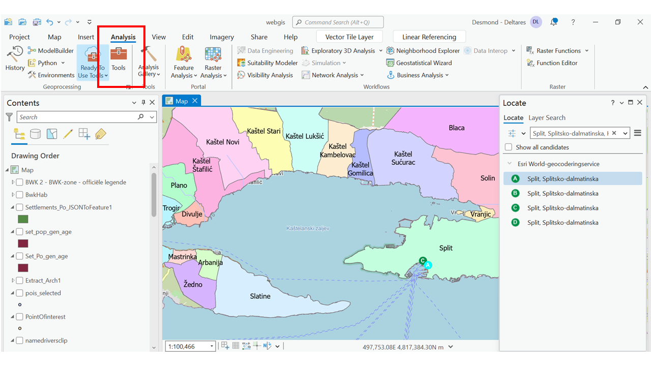
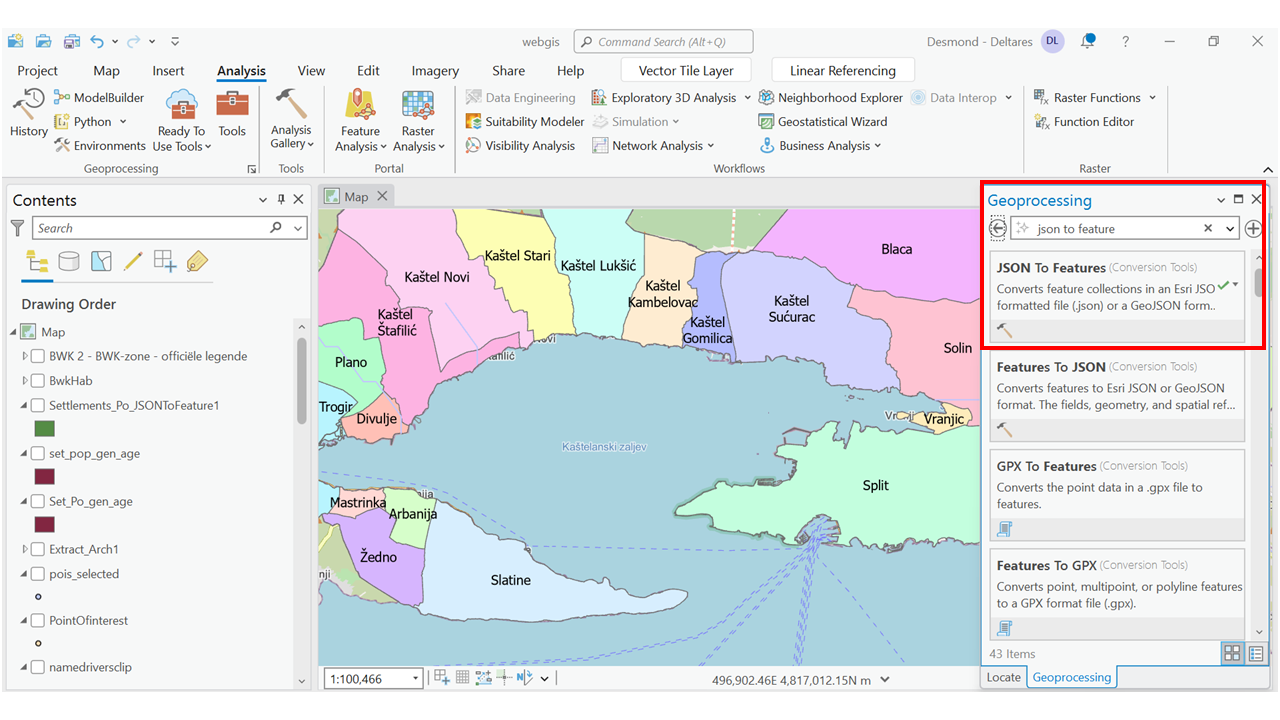
Step 3: Converting JSON to Feature Class in ArcGIS Pro
- Open **ArcGIS Pro**.
- Go to Analysis → Tools
- And search for **"JSON to Features"*.
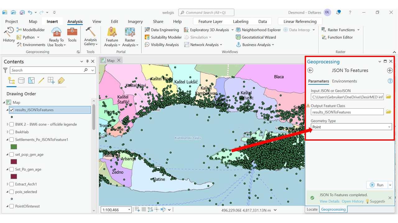
- Select the **downloaded JSON file** as input. And click run.By default, the geometry type is set to Polygon. Remember to change it to point
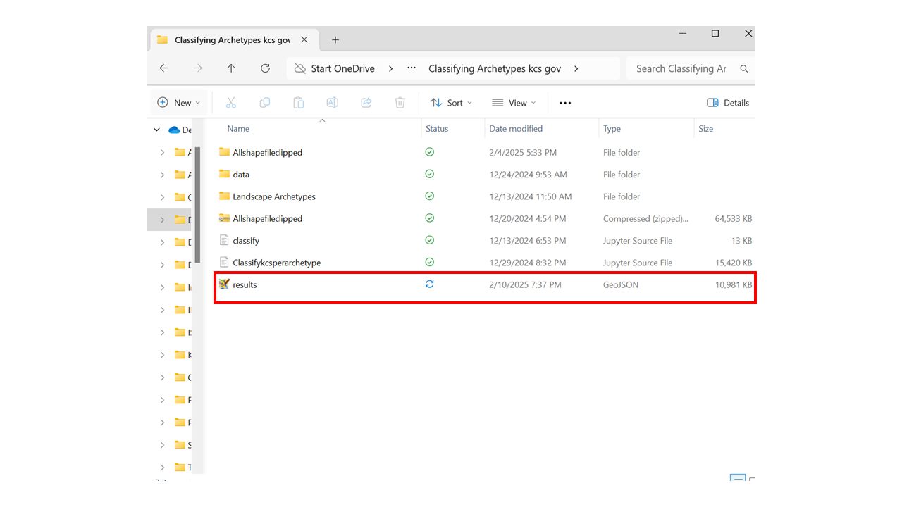
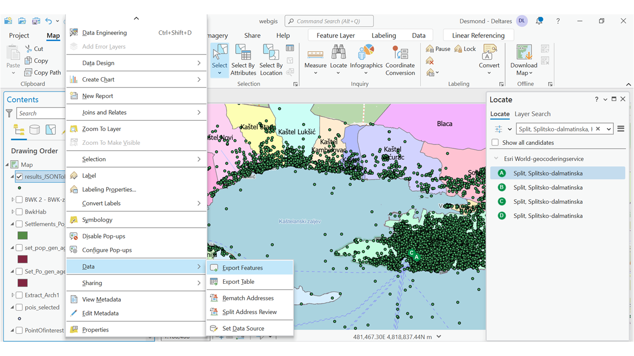
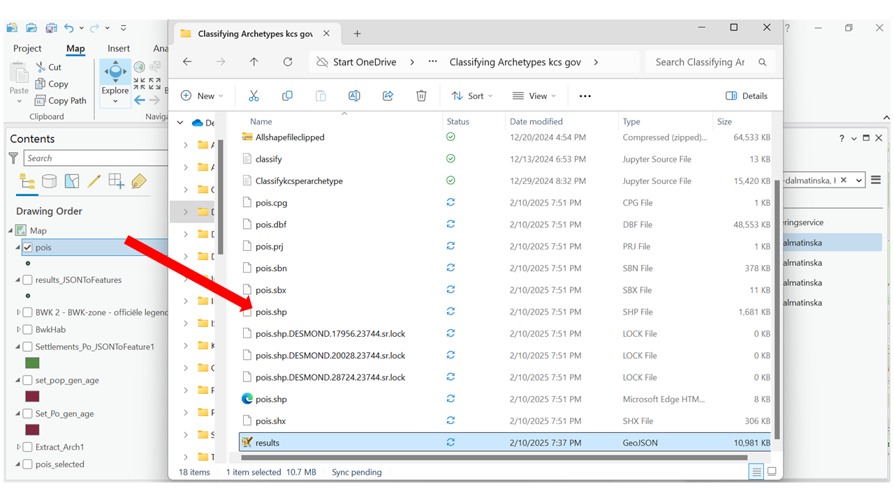
- Export as **Shapefile (.shp)**.
- You should now see your (.shp) poi data in where you saved it with other file extensions**.
You can now import this data into earth engine for the spatial aggregation. You can consult previous guide to learn about how to import data into Earth engine as an asset.
Now that we have **ingested the data into Google Earth Engine (GEE)**, we will proceed with **spatial aggregation** in the next section.
Step 1: Spatial Aggregation of Points of Interest (POIs)
Now that we have **inspected and validated** the **Foursquare dataset**, we proceed to integrate it with the **settlements dataset** using **spatial aggregation** in **Google Earth Engine (GEE)**.
In this step, we will **aggregate** POI data by their **category levels** into the **settlement boundaries**, allowing us to assess how different **socioeconomic activities** are distributed.
Step 2: Load the Required Datasets
The following script loads:
- Settlement Boundaries: This dataset contains polygons representing **individual settlements**.
- POI Dataset: This dataset contains **Points of Interest**, classified into **category levels**.
// Load the settlements dataset
var settlements = ee.FeatureCollection("projects/ee-desmond/assets/desirmed/settlements_population_with_gender_age");

// Load the Point of Interest (POI) dataset
var poiDataset = ee.FeatureCollection('projects/ee-desmond/assets/desirmed/PointOfinterest');

// Print dataset structure
print(" Settlement Dataset:", settlements);
print(" POI Dataset:", poiDataset);
The **print() function** is used here to inspect the datasets before aggregation. This ensures that the **attribute structure** and **geometries** are correct before proceeding.
Step 3: Aggregating POIs into Settlements
The **aggregation process** involves the following steps:
- For each settlement, filter out **POIs that fall within its boundary**.
- Use the
aggregate_histogram()function to count POIs by category. - Add the aggregated counts as **new properties** to the settlement dataset.
// Integrate POIs into settlements
var enhancedSettlementsWithPOI = settlements.map(function(feature) {
// Filter POIs within the settlement boundary
var poiInFeature = poiDataset.filterBounds(feature.geometry());
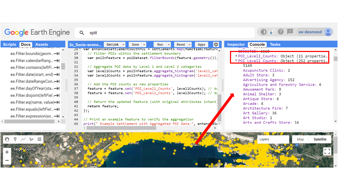
// Aggregate POI data by Level 1 and Level 2 categories
var level1Counts = poiInFeature.aggregate_histogram('level1_cat'); // Counts by Level 1 categories
var level2Counts = poiInFeature.aggregate_histogram('level2_cat'); // Counts by Level 2 categories
// Add the POI counts as new properties
feature = feature.set('POI_Level1_Counts', level1Counts); // Add Level 1 POI counts
feature = feature.set('POI_Level2_Counts', level2Counts); // Add Level 2 POI counts
// Return the updated feature (with original attributes intact)
return feature;
});
// Print an example feature to verify the aggregation
print(" Example Settlement with Aggregated POI Data:", enhancedSettlementsWithPOI.first());
- The **
map()function** loops over each settlement feature. - The **
filterBounds()function** extracts only the POIs that fall within the **settlement boundary**. - The **
aggregate_histogram()function** computes a **frequency count** of POIs per category. - The **aggregated values** are stored as **new attributes** under:
POI_Level1_Counts: High-level POI category counts (e.g., Food, Education).POI_Level2_Counts: More detailed breakdown of POI categories (e.g., Restaurants, Schools).
Once the aggregation is complete, each **settlement feature** will contain new attributes summarizing the type/categories of KCS and the **number of that per each category within its boundary**.
Example Output:
{
  "type": "Feature",
  "properties": {
    "name": "Bruges",
    "population": 117000,
    "POI_Level1_Counts": {
      "Food & Drink": 125,
      "Education": 42,
      "Retail": 87
    },
    "POI_Level2_Counts": {
      "Restaurants": 89,
      "Cafes": 30,
      "Schools": 42,
      "Supermarkets": 50
    }
  },
  "geometry": { "type": "Polygon", "coordinates": [...] }
}
This output helps in **identifying economic hubs** within the landscape. For example, a settlement with a **high density of restaurants and cafes** might indicate a **commercial center**, while an area with **many schools and libraries** could represent an **educational zone**.
This spatial aggregation allows us to **identify clusters of key community systems** within each settlement, providing valuable insights into their **distribution and density**. By analyzing these clusters, we can:
- Quantify the **availability and accessibility** of essential services within a given settlement.
- Evaluate the **exposure and vulnerability** of community assets to various environmental and socio-economic risks through **overlay analysis** with hazard datasets.
- Assess how existing KCS can support or limit the **development and implementation of Nature-based Solutions (NbS)** for climate resilience and urban planning.
You can see that the first asset "settlements_population_with_gender_age" is used as the defined boundary this time. The reason is that this is already a datasets with extra info about each settlement within the SDC. We do not cover how to make this dataset in this guide. But we have made it publicly accessible. Also if you don't specify an area within the list of settlemes, Earth engine by default will compute the aggreage on the first settlement 'Hvar'. This settlement have NO point of interest. So you need to first apply a filter to specify different area. We leave that to you.
Governance Domain
Governance is a crucial aspect of landscape characterization within the Desirmed Project. It provides insights into decision-making structures, land management, environmental protection, and policy influence. Understanding governance layers helps in:
- Defining territorial boundaries for analysis and policymaking.
- Assessing the institutional capacity to manage natural hazards and resilience strategies.
- Linking governance structures to landscape risks, ecosystem services, and socio-economic factors.
Where does governance fit into Desirmed?
- Governance influences land-use decisions, urban expansion, and environmental conservation.
- It defines jurisdictional authority for risk management (e.g., flood control, protected areas).
- It is linked to **climate risk impact chains** – where policy frameworks dictate the implementation of Nature-based Solutions (NbS).
Data Sources for Governance Layers
We will use various governance datasets to map political and administrative structures relevant to **landscape characterization**.
- Administrative Boundaries: Define the **national, regional, and local** governance units.
- Statistical Units (NUTS & LAU): Used for socio-economic and policy analysis.
- Basic Services: Includes public facilities such as **hospitals and transport hubs**.
- River Basin Authorities: Important for **water resource management**.
- Protected Areas: Biodiversity conservation zones such as **Natura 2000 sites**.
Accessing Governance Data
The datasets we will use are sourced from various **European Commission & EU environmental agencies**:
- Local Administrative Units (LAU)
- National Boundaries
- NUTS Statistical Units
- Catchment Characterization (River Basins)
- Marine Protected Areas
- Hydrosheds
For this tutorial, we will not go through all the steps in downloading these layers
We will rather demonstrate clipping a governance dataset to a defined **Region of Interest (ROI)** – in this case, Split-Dalmatia County.
Clipping a Governance Dataset in ArcGIS Pro
Once we have downloaded the governance unit layers, we need to clip them to our study area.
Steps to Clip a Dataset
- Open ArcGIS Pro and create a new project.
- Add the governance dataset (e.g., Local Administrative Units).
- Add the Split-Dalmatia County boundary as the **clip feature**.
- Go to Analysis → Tools, search for **Clip**.
- Set the governance layer as the Input Feature.
- Set the Split-Dalmatia boundary as the Clip Feature.
- Run the tool and save the output to your workspace.
Efficient Processing with ModelBuilder
If you plan to work with multiple governance layers, **ModelBuilder** provides a more efficient workflow.
To help you even understand the effienciency of the modelbuilder, we make a simple illustration here with the Hydrosheds dataset
- Go to Hydroshed website
- Look for Europe and Middle East as **Extent** and click on the downloads.
- You can download the entire Europe and Middle East dataset as Geodatabase file format.
- Import the **HydroRIVERS dataset** into **ArcGIS Pro**.
- Add the **Split-Dalmatia County boundary** to your project.
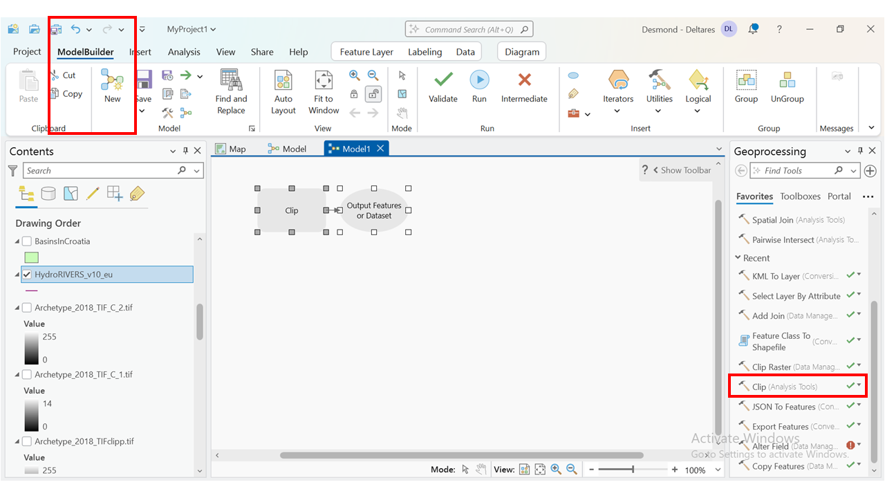
- Click on the Analysis button in the ArcGIS toolbar.
- Find and click on ModelBuilder to open the interface.
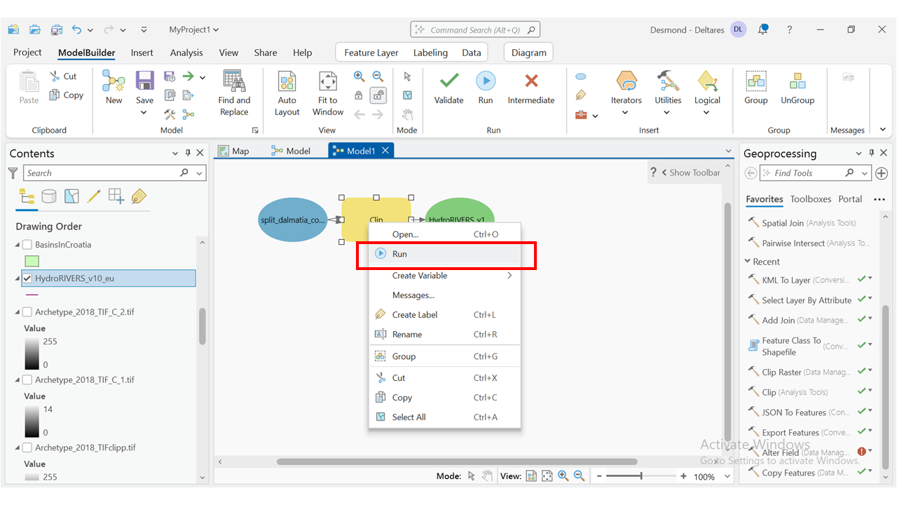
- Click on **Tools** to open the **Geoprocessing Search Bar**.
- Search for **Clip** and **drag it into your model canvas**.
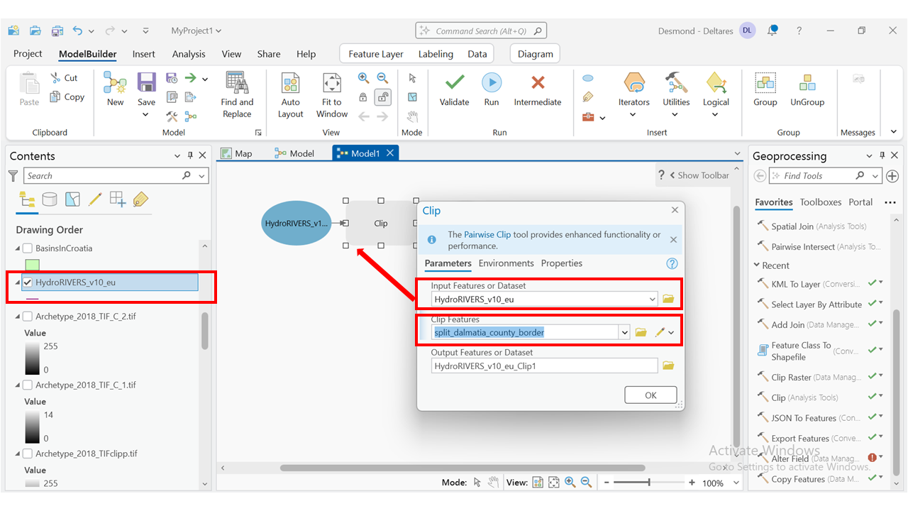
- Drag your **HydroRIVERS dataset** into the **Input Features**.
- Drag your **Split-Dalmatia County boundary** into the **Clip Features**.
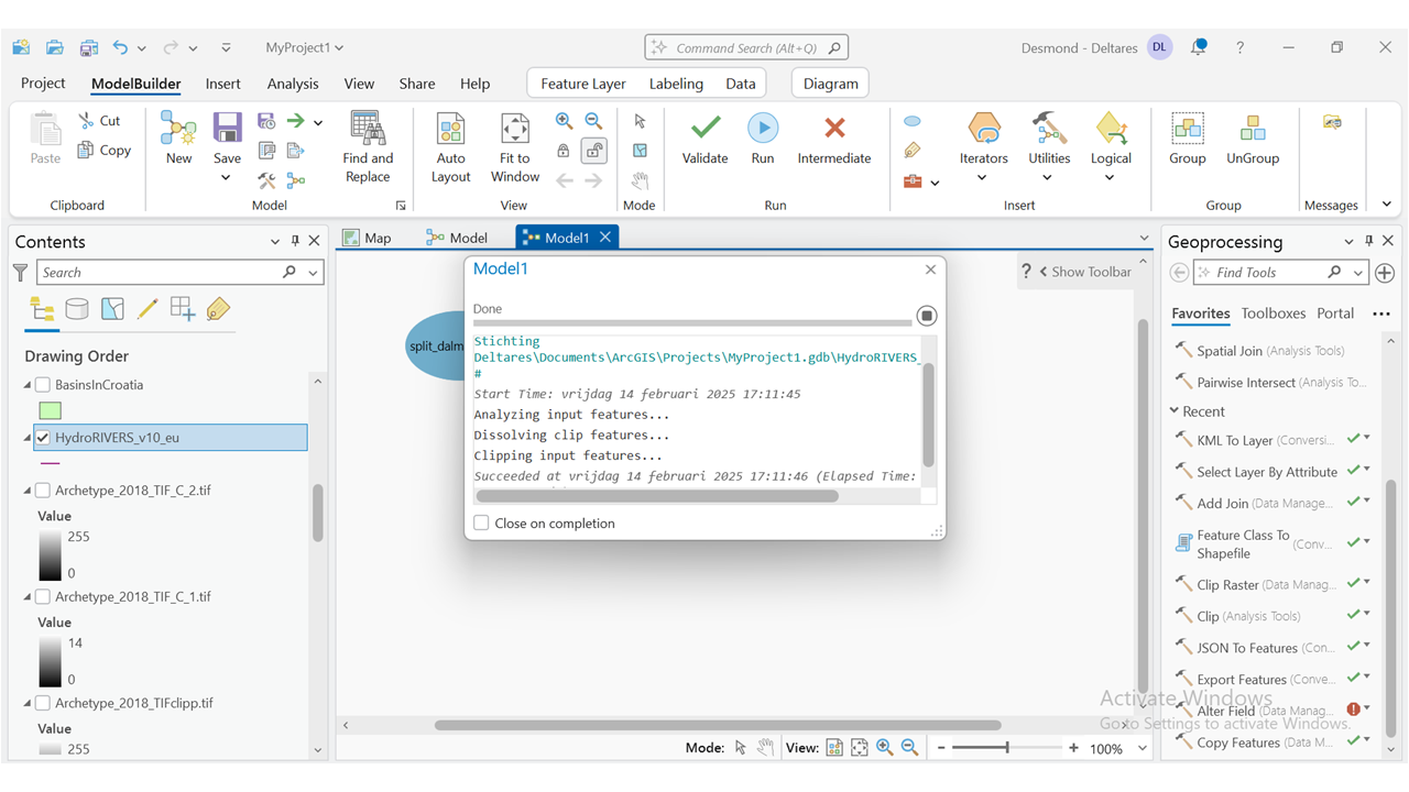
- Right-click on the **Clip tool** and select **Run**.
- Ensure that the run is complete 100% with no **Error**.
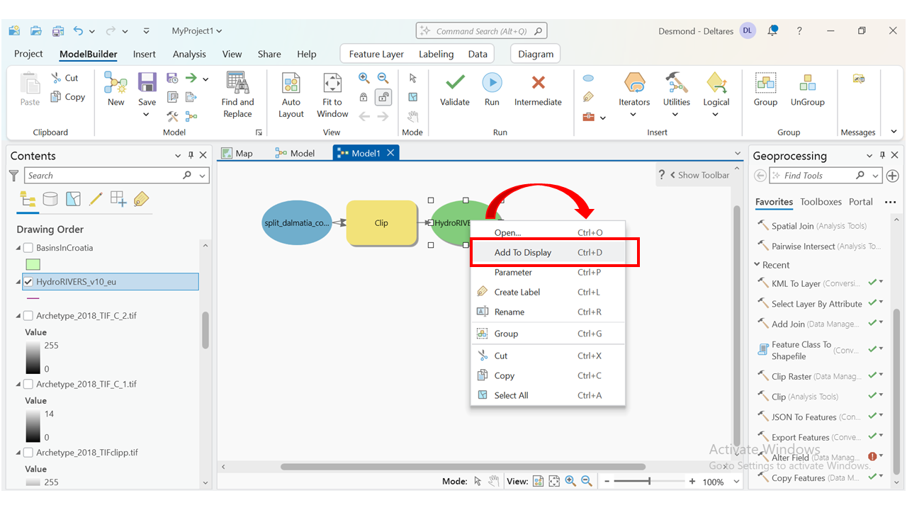
- Once the process is complete, **right-click on the new clipped feature** and select **Add to Display**.
- Inspect the **attribute table** to determine relevant fields.
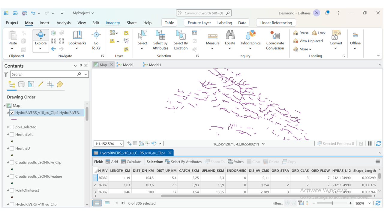
Why Inspect the Attributes?
- To check if the dataset includes **river management authorities**.
- To determine if additional **data updates** are required.
Advantages of ModelBuilder:
- Automates **batch processing** of multiple layers.
- Ensures **consistency** in data extraction.
- Saves time by running multiple processes in one workflow.
Pre-Processed Governance Data
For convenience, we have downloaded, processed, and clipped all governance layers for the Split-Dalmatia region.
➡ Download Processed Governance Data Here
Using the Exported Python Model
We have also exported the **ModelBuilder workflow** as a Python script. This allows you to automate similar tasks in different regions.
How to Use the Python Script
- Ensure **ArcGIS Pro with arcpy** is installed.
- Update the **input dataset paths** in the script.
- Run the script in **Python or ArcGIS Pro's Python window**.
Breaking Down the Script
Below is an overview of how the script works and how you can modify it for your own datasets.
1. Setting Up the Environment
# Import ArcPy
import arcpy

# Enable overwrite
arcpy.env.overwriteOutput = True
- This imports the **ArcPy** library, used for geospatial processing in ArcGIS.
- It enables **overwriteOutput**, allowing files to be replaced if they already exist.
2. Defining Input and Output Data
# Define input features
governance_layer = "C:\\Data\\Governance\\Local_Admin_Units.shp"
clip_boundary = "C:\\Data\\Regions\\Split_Dalmatia.shp"

# Define output path
clipped_output = "C:\\ProcessedData\\Governance_Clipped.shp"
- Modify **governance_layer** to match your downloaded dataset.
- Update **clip_boundary** with the boundary of your region.
- Set **clipped_output** to where the processed file should be saved.
3. Running the Clipping Tool
# Perform the clip operation
arcpy.analysis.Clip(in_features=governance_layer,
                    clip_features=clip_boundary,
                    out_feature_class=clipped_output)
- This line **clips the governance data** to the region.
- It ensures that only relevant administrative units are kept.
4. Running the Script
To run the script:
- Open **ArcGIS Pro**.
- Go to **Python Window** or use a **Python IDE (e.g., Jupyter, PyCharm).**
- Execute the script to process the governance layers.
Download the Full Script
To access the complete Python script and modify it for your own project:
➡ Download the Python Clipping Script Here
EUNIS Dataset Creation
The EUNIS habitat classification system is a vital tool for understanding habitat types across Europe, supporting biodiversity monitoring, conservation planning, and ecosystem-based management. By standardizing habitat classification, EUNIS provides a framework for consistent ecological assessments. To our knowledge, there isnt a unified EUNIS habitat map for the entire europe except smaller polygon shapes that exist as properties in other datasets. This is why we create one for the purpose of this study. While some EUNIS maps exist, they are often based on older datasets and may not reflect recent land use changes or provide adequate detail for dynamic regions.
Our workflow builds upon the foundational work conducted in the RESTCOAST project. In Resct-coast, researchers used corine land cover data to derive EUNIS classifications using 1-to-1 tabular translation. But this create some limitations that we aim to address using a more detailed landuse/cover classes at higher resolution.
Shortcomings of the RESTCOAST Approach
- **Outdated Classifications:** Reliance on classification code from 2012 limit the ability to capture recent habitats.
- **Overlapping Geometries:** Challenges in addressing overlapping polygons resulted in ambiguities in habitat delineations and area calculations.
- **Limited EUNIS Class Translation:** Not all available LULC classes were fully mapped to the comprehensive list of EUNIS habitat types, potentially leaving some habitats underrepresented.
Improvements in This Workflow
To overcome these limitations, this workflow incorporates the following enhancements:
- **Use of the detailed and higher resolution Datasets:** The 2018 coastal LULC datasets provide better alignment with current ecological realities and landscape changes.
- **Refined Crosswalk Mapping:** A complete translation table, including all 71 land use/cover types, ensures thorough and accurate habitat mapping. Access the full translation table we developed here.
- **Advanced Handling of Overlaps:** Overlapping geometries are resolved ensuring consistency in habitat delineation.
- **Scalability and Flexibility:** Leveraging GEE allows us to handle large datasets, perform complex spatial analyses, and generate high-resolution EUNIS maps dynamically.
Our methodology ensures a more robust and comprehensive EUNIS dataset, addressing past limitations and providing better support for conservation efforts.
Land Use to EUNIS Crosswalk
To translate LULC data into EUNIS habitat types, a crosswalk table is employed. This table maps each LULC class to its corresponding EUNIS code, ensuring consistency and ecological relevance. Below is a snippet of the translation:
| Land Use Code | Land Use Description | EUNIS Numeric | EUNIS Code | EUNIS Description |
|---|---|---|---|---|
| 11110 | Continuous urban fabric (IMD >= 80%) | 1 | J1 | Buildings of cities, towns, and villages |
| 11120 | Dense urban fabric (IMD >= 30-80%) | 2 | J1.2 | Residential buildings of villages and urban peripheries |
| 11130 | Low density fabric (IMD < 30%) | 3 | J2 | Low density buildings |
| 11210 | Industrial, commercial, public, and military units | 4 | J4 | Transport networks and other hard-surfaced areas |
| 11220 | Nuclear energy plants and associated land | 5 | J4.5 | Hard-surfaced areas of ports |
| 12100 | Road networks and associated land | 6 | J4.4 | Airport runways and aprons |
| 12310 | Cargo port | 5 | J4.5 | Hard-surfaced areas of ports |
| 12320 | Passenger port | 5 | J4.5 | Hard-surfaced areas of ports |
| 31100 | Agro-forestry | 19 | V6 | Tree dominated man-made habitats |
| 63200 | Burnt areas (except burnt forest) | 40 | U5 | Miscellaneous inland habitats usually with very sparse or no vegetation |
| 84100 | Open sea | 57 | MC5 | Circalittoral sand |
Access the full list of EUNIS habitat classifications for detailed descriptions and additional information on habitat types.
You can also access the full eunis tranlation code for coastal areas here.
Some EUNIS codes repeat for different land use classes, such as port-related classes (e.g., cargo port, passenger port) mapping to J4.5. This repetition reflects the shared ecological characteristics of these land uses. However, it also underscores the need for careful validation to ensure that such overlaps do not introduce ambiguities into habitat assessments. From a special point of view, we have added a 2012 Eunis habitat map just to compare changes. This helps to also validate if a change of a classified eunis class make sense or not
We will proceed to outline the step-by-step process for creating a EUNIS habitat map.
Step 1: Define Land Cover Datasets
To start, we need to define the datasets that represent land cover for the years 2012 and 2018. These datasets will form the basis of our EUNIS habitat classification.
// Define the land cover datasets
var landCoverYears = {
  '2012': ee.FeatureCollection('projects/ee-desmond/assets/lulc2012_Croatiafinal'),
  '2018': ee.FeatureCollection('projects/ee-desmond/assets/lulc2018_Croatiafinal')
};
This step initializes an object containing the FeatureCollections for the two datasets. Each dataset represents the land cover of Croatia for a specific year.
Step 2: Define the Crosswalk Mapping
In this step, we define how land cover classes from the datasets are translated into EUNIS habitat codes. This mapping is essential for accurate reclassification.
// Define the crosswalk mapping from land cover classes to EUNIS habitats
var landCoverToEunisNumeric = {
  11110: 1,  // J1 - Buildings of cities, towns, and villages
  11120: 2,  // J1.2 - Residential buildings of villages and urban peripheries
  11130: 3,  // J2 - Low density buildings
  11210: 4,  // J4 - Transport networks and other hard-surfaced areas
  11220: 5,  // J4.5 - Hard-surfaced areas of ports
  12100: 6,  // J4.4 - Airport runways and aprons
  12200: 7,  // J3 - Extractive industrial sites
  12310: 5,  // J4.5 - Hard-surfaced areas of ports
  12320: 5,  // J4.5 - Hard-surfaced areas of ports
  12330: 5,  // J4.5 - Hard-surfaced areas of ports
  12340: 5,  // J4.5 - Hard-surfaced areas of ports
  12350: 5,  // J4.5 - Hard-surfaced areas of ports
  12360: 5,  // J4.5 - Hard-surfaced areas of ports
  12370: 5,  // J4.5 - Hard-surfaced areas of ports
  12400: 6,  // J4.4 - Airport runways and aprons
  13110: 7,  // J3 - Extractive industrial sites
  13120: 8,  // J6 - Waste deposits
  13130: 9,  // J1.6 - Urban and suburban construction and demolition sites
  14000: 10,	//J2.6-2012	Disused rural constructions
  21100: 11,	//E2.6-2012'	Heavily fertilised grassland, including sports fields and grass lawns
  21200: 12,	//I1.1	Intensive unmixed crops
  22100: 13,	//J2.43-2012	Greenhouses
  22200: 14,	//V5	Shrub plantations
  23100: 15,	//T24	Olea europaea-Ceratonia siliqua forest
  23200: 16,	//	//B15	Bare tilled, fallow or recently abandoned arable land
  23300:	17,	//	V12	Mixed crops of market gardens and horticulture
  23400:	18,	//	V13	Arable land with unmixed crops grown by low-intensity agricultural methods
  31100:	19,	//	V6	Tree dominated man-made habitats
  31200:	20,	//	T1	Deciduous broadleaved forest
  31300:	21,	//	T29	Broadleaved evergreen plantation of non site-native trees
  32100:	22,	//	T3	Coniferous forest
  32200:	23,	//	T3N	Coniferous plantation of site-native trees
  33100:	24,	//	G4-2012	Mixed deciduous and coniferous woodland
  33200:  25,	//	G4.F-2012	Mixed forestry plantations
  34000:	26,	//	T41	Early-stage natural and semi-natural forest and regrowth
  35000:	27,	//	T42	Early-stage natural and semi-natural forest and regrowth
  36000:	28,	//	T43	Recently felled areas
  41000:	29,	//	V3	Artificial grasslands and herb dominated habitats
  42100:	30,	//	R2	Mesic grasslands
  42200:	31,	//	R4	Alpine and subalpine grasslands
  51000:	32,	//	S4	Temperate shrub heathland
  52000:	33,	//	S2	Arctic, alpine and subalpine scrub
  53000:	34,	//	F5	Maquis, arborescent matorral, and thermo-Mediterranean brushes
  61100:	35,	//	U2	Screes
  61200:	35,	//	U2	Screes
  62111:	36,	//	N1	Coastal dunes and sandy shores
  62112:	36,	//	N1	Coastal dunes and sandy shores
  62120:	37,	//	N14	Mediterranean, Macaronesian and Black Sea shifting coastal dune
  62200:	38,	//	C3.6-2012	Unvegetated or sparsely vegetated shores with soft or mobile sediments
  63110:	39,	//	U3	Inland cliffs, rock pavements and outcrops
  63120:	39,	//	U3	Inland cliffs, rock pavements and outcrops
  63200:	40,	//	U5	Miscellaneous inland habitats usually with very sparse or no vegetation
  63300:	41,	//	U4	Snow or ice-dominated habitats
  71100:	42,	//	D2-2012	Valley mires, poor fens and transition mires
  71210:	43,	//	D1	Raised and blanket bogs
  71220:	43,	//	D1	Raised and blanket bogs
  72100:	44,	//	MA2	Littoral biogenic habitat
  72200:	45,	//	J5.1	Highly artificial saline and brackish standing waters
  72300:	46,	//	MA5	Littoral sand
  81100:	47,	//	C2	Surface running waters
  81200:	48,	//	J5-2012	Highly artificial man-made waters and associated structures
  81300:	49,	//	C2.5-2012	Temporary running waters
  82100:	50,	//	C1	Surface standing waters
  82200:	51,	//	J5.3-2012	Highly artificial non-saline standing waters
  82300:	52,	//	J5.32-2012	Intensively managed fish ponds
  82400:	53,	//	J5.34-2013	Standing waterbodies of extractive industrial sites with extreme chemistry
  83100:	54,	//	X02-2012	Saline coastal lagoons
  83200:	55,	//	X01	Estuaries
  83300:	56,	//	MB1	Infralittoral rock
  84100:	57,	//	MC5	Circalittoral sand
  84200:	58,	//	MB5	Infralittoral sand


};
This object maps numeric land cover codes to their corresponding EUNIS numeric codes. Each mapping represents a habitat type, allowing us to translate land cover data into the EUNIS classification system.
Step 3: Define the EUNIS Properties
Here, we assign properties like color and descriptions to EUNIS habitat types. This enhances visualization and understanding of the output.
// Define the EUNIS properties mapping
  var eunisNumericMapping = {
    1: {eunisCode: 'J1', color: '#b22222', description: 'Buildings of cities, towns, and villages'}, // Deep red for urban areas
    2: {eunisCode: 'J1.2', color: '#ff4500', description: 'Residential buildings of villages and urban peripheries'}, // Orange-red
    3: {eunisCode: 'J2', color: '#ffa07a', description: 'Low density buildings'}, // Light coral for suburban areas
    4: {eunisCode: 'J4', color: '#8b4513', description: 'Transport networks and other hard-surfaced areas'}, // Saddle brown for roads
    5: {eunisCode: 'J4.5', color: '#d2691e', description: 'Hard-surfaced areas of ports'}, // Chocolate brown
    6: {eunisCode: 'J4.4', color: '#808080', description: 'Airport runways and aprons'}, // Gray for airstrips
    7: {eunisCode: 'J3', color: '#556b2f', description: 'Extractive industrial sites'}, // Dark olive green for industrial land
    8: {eunisCode: 'J6', color: '#a0522d', description: 'Waste deposits'}, // Sienna for waste areas
    9: {eunisCode: 'J1.6', color: '#d2b48c', description: 'Urban and suburban construction and demolition sites'}, // Tan
    10: {eunisCode: 'J2.6-2012', color: '#deb887', description: 'Disused rural constructions'}, // Burlywood
    11: {eunisCode: 'E2.6-2012', color: '#32cd32', description: 'Heavily fertilised grassland, including sports fields and grass lawns'}, // Lime green for managed grass
    12: {eunisCode: 'I1.1', color: '#adff2f', description: 'Intensive unmixed crops'}, // Green-yellow for intensive crops
    13: {eunisCode: 'J2.43-2012', color: '#ff7f50', description: 'Greenhouses'}, // Coral for greenhouses
    14: {eunisCode: 'V5', color: '#8fbc8f', description: 'Shrub plantations'}, // Dark sea green for shrubs
    15: {eunisCode: 'T24', color: '#228b22', description: 'Olea europaea-Ceratonia siliqua forest'}, // Forest green
    16: {eunisCode: 'B15', color: '#f4a460', description: 'Bare tilled, fallow or recently abandoned arable land'}, // Sandy brown
    17: {eunisCode: 'V12', color: '#ffe4b5', description: 'Mixed crops of market gardens and horticulture'}, // Moccasin
    18: {eunisCode: 'V13', color: '#f0e68c', description: 'Arable land with unmixed crops grown by low-intensity agricultural methods'}, // Khaki
    19: {eunisCode: 'V6', color: '#6b8e23', description: 'Tree dominated man-made habitats'}, // Olive drab
    20: {eunisCode: 'T1', color: '#008000', description: 'Deciduous broadleaved forest'}, // Green for forest
    21: {eunisCode: 'T29', color: '#2e8b57', description: 'Broadleaved evergreen plantation of non site-native trees'}, // Sea green
    22: {eunisCode: 'T3', color: '#3cb371', description: 'Coniferous forest'}, // Medium sea green
    23: {eunisCode: 'T3N', color: '#66cdaa', description: 'Coniferous plantation of site-native trees'}, // Medium aquamarine
    24: {eunisCode: 'G4-2012', color: '#20b2aa', description: 'Mixed deciduous and coniferous woodland'}, // Light sea green
    25: {eunisCode: 'G4.F-2012', color: '#5f9ea0', description: 'Mixed forestry plantations'}, // Cadet blue
    26: {eunisCode: 'T41', color: '#4682b4', description: 'Early-stage natural and semi-natural forest and regrowth'}, // Steel blue
    27: {eunisCode: 'T42', color: '#87cefa', description: 'Early-stage natural and semi-natural forest and regrowth'}, // Light sky blue
    28: {eunisCode: 'T43', color: '#d3d3d3', description: 'Recently felled areas'}, // Light gray
    29: {eunisCode: 'V3', color: '#7cfc00', description: 'Artificial grasslands and herb dominated habitats'}, // Lawn green
    30: {eunisCode: 'R2', color: '#006400', description: 'Mesic grasslands'}, // Dark green
    31: {eunisCode: 'R4', color: '#556b2f', description: 'Alpine and subalpine grasslands'}, // Dark olive green
    32: {eunisCode: 'S4', color: '#8b0000', description: 'Temperate shrub heathland'}, // Dark red
    33: {eunisCode: 'S2', color: '#00008b', description: 'Arctic, alpine, and subalpine scrub'}, // Dark blue
    34: {eunisCode: 'F5', color: '#b0c4de', description: 'Maquis, arborescent matorral, and thermo-Mediterranean brushes'}, // Light steel blue
    35: {eunisCode: 'U2', color: '#708090', description: 'Screes'}, // Slate gray
    36: {eunisCode: 'N1', color: '#fa8072', description: 'Coastal dunes and sandy shores'}, // Salmon
    37: {eunisCode: 'N14', color: '#f08080', description: 'Mediterranean, Macaronesian and Black Sea shifting coastal dune'}, // Light coral
    38: {eunisCode: 'C3.6-2012', color: '#add8e6', description: 'Unvegetated or sparsely vegetated shores with soft or mobile sediments'}, // Light blue
    39: {eunisCode: 'U3', color: '#dda0dd', description: 'Inland cliffs, rock pavements and outcrops'}, // Plum
    40: {eunisCode: 'U5', color: '#ba55d3', description: 'Miscellaneous inland habitats usually with very sparse or no vegetation'}, // Medium orchid
    41: {eunisCode: 'U4', color: '#9400d3', description: 'Snow or ice-dominated habitats'}, // Dark violet
    42: {eunisCode: 'D2-2012', color: '#00ced1', description: 'Valley mires, poor fens and transition mires'}, // Dark turquoise
    43: {eunisCode: 'D1', color: '#4682b4', description: 'Raised and blanket bogs'}, // Steel blue
    44: {eunisCode: 'MA2', color: '#6495ed', description: 'Littoral biogenic habitat'}, // Cornflower blue
    45: {eunisCode: 'J5.1', color: '#1e90ff', description: 'Highly artificial saline and brackish standing waters'}, // Dodger blue
    46: {eunisCode: 'MA5', color: '#ffdab9', description: 'Littoral sand'}, // Peach puff
    47: {eunisCode: 'C2', color: '#4169e1', description: 'Surface running waters'}, // Royal blue
    48: {eunisCode: 'J5-2012', color: '#8b0000', description: 'Highly artificial man-made waters and associated structures'}, // Dark red
    49: {eunisCode: 'C2.5-2012', color: '#5f9ea0', description: 'Temporary running waters'}, // Cadet blue
    50: {eunisCode: 'C1', color: '#00bfff', description: 'Surface standing waters'}, // Deep sky blue
    51: {eunisCode: 'J5.3-2012', color: '#1e90ff', description: 'Highly artificial non-saline standing waters'}, // Dodger blue
    52: {eunisCode: 'J5.32-2012', color: '#ff4500', description: 'Intensively managed fish ponds'}, // Orange-red
    53: {eunisCode: 'J5.34-2013', color: '#228b22', description: 'Standing waterbodies of extractive industrial sites with extreme chemistry'}, // Forest green
    54: {eunisCode: 'X02-2012', color: '#87ceeb', description: 'Saline coastal lagoons'}, // Sky blue
    55: {eunisCode: 'X01', color: '#00008b', description: 'Estuaries'}, // Dark blue
    56: {eunisCode: 'MB1', color: '#6baed6', description: 'Infralittoral rock'}, // Steel blue
    57: {eunisCode: 'MC5', color: '#e6f2ff', description: 'Circalittoral sand'}, // Blue violet
    58: {eunisCode: 'MB5', color: '#2171b5', description: 'Infralittoral sand'} // Light steel blue
  };
Each EUNIS code is assigned a color and description. This is useful for visualization and interpretation of the classified datasets.
Step 4: Reclassify Land Cover to EUNIS
Now, we write a function to reclassify the land cover dataset into EUNIS habitats based on the mapping we defined earlier.
// Function to reclassify land cover data into EUNIS numeric codes
var reclassifyToEunis = function(dataset, codeField, mapping) {
  var mappingKeys = Object.keys(mapping).map(Number); // Input land cover class codes as numbers
  var mappingValues = Object.keys(mapping).map(function(key) {
    return mapping[key]; // Extract corresponding EUNIS numeric codes
  });

  return dataset.remap(
    mappingKeys,  // CORINE codes as input
    mappingValues // Corresponding EUNIS numeric codes
  );
};
This function accepts a dataset, a code field, and the mapping object. It uses the remap function to reclassify the dataset based on the mapping.
Step 5: Visualize the Reclassified Dataset
We create another function to style the reclassified EUNIS image for visualization in Google Earth Engine.
// Function to style the reclassified EUNIS image
var styleEunisImage = function(image) {
  var palette = Object.keys(eunisNumericMapping).map(function(key) {
    return eunisNumericMapping[key].color; // Extract EUNIS color values
  });

  return image.visualize({
    min: 1,
    max: 58, // Adjust range based on EUNIS numeric codes
    palette: palette // Apply palette for EUNIS visualization
  });
};
This function applies a color palette to the reclassified dataset for better visualization. The palette is derived from the EUNIS properties defined earlier.
Step 6: Define Croatia Coastal Boundaries
We define the geographic bounds of Croatia's coastal regions to limit the analysis to the relevant area.
// Define Croatia's coastal bounds
var croatiaCoastalBounds = ee.Geometry.Polygon([
  [13.5, 44.0], [18.5, 44.0], [18.5, 42.0], [13.5, 42.0], [13.5, 44.0]
]);
This polygon defines the region of interest, focusing the analysis on Croatia's coastal area and excluding inland or irrelevant regions.
Step 7: Reclassify and Style the 2012 Dataset
Using the reclassification and visualization functions, we process the 2012 land cover dataset.
// Reclassify and style 2012 dataset
var reclassified2012 = reclassifyToEunis(
  landCoverYears['2012'].filterBounds(croatiaCoastalBounds).reduceToImage(['CODE_5_12'], ee.Reducer.first()),
  'CODE_5_12',
  landCoverToEunisNumeric
);

Map.addLayer(reclassified2012, {
  min: 1,
  max: 58,
  palette: Object.keys(eunisNumericMapping).map(function(key) {
    return eunisNumericMapping[key].color;
  })
}, 'EUNIS 2012');
This step filters, reclassifies, and visualizes the 2012 dataset for Croatia's coastal regions.
Step 8: Reclassify and Style the 2018 Dataset
We repeat the process for the 2018 dataset, ensuring consistency in approach and visualization.
// Reclassify and style 2018 dataset
var reclassified2018 = reclassifyToEunis(
  landCoverYears['2018'].filterBounds(croatiaCoastalBounds).reduceToImage(['CODE_5_18'], ee.Reducer.first()),
  'CODE_5_18',
  landCoverToEunisNumeric
);

Map.addLayer(reclassified2018, {
  min: 1,
  max: 58,
  palette: Object.keys(eunisNumericMapping).map(function(key) {
    return eunisNumericMapping[key].color;
  })
}, 'EUNIS 2018');
The 2018 dataset is processed in the same way, enabling direct comparison with the 2012 dataset.
Now that the 2018 dataset is visualized, comparisons between 2012 and 2018 are possible.
Step 9: Create a Chart for Comparing EUNIS Areas
strong>Comparing habitat areas across years provides insights into ecological changes. This is done by computing areas of each EUNIS class and displaying them in bar and pie charts for better visualization.
// Function to compute EUNIS areas
var computeEunisAreas = function(image, year, geometry) {
  var areaImage = ee.Image.pixelArea().divide(1e6).addBands(image.rename('class')); // Area in km²
  var areas = areaImage.reduceRegion({
    reducer: ee.Reducer.sum().group({
      groupField: 1,
      groupName: 'class'
    }),
    geometry: geometry,
    scale: 100,
    maxPixels: 1e13
  });
  return ee.List(areas.get('groups')).map(function(item) {
    var areaDict = ee.Dictionary(item);
    return ee.Feature(null, {
      'class': ee.Number(areaDict.get('class')),
      'area': ee.Number(areaDict.get('sum')),
      'year': year
    });
  });
};
The computed areas for both 2012 and 2018 datasets are visualized in a bar chart for direct comparison.
Step 10: Export the Reclassified Data
To facilitate further analysis or sharing, the reclassified datasets for 2012 and 2018 are exported in raster and vector formats. These exports allow users to inspect and validate the data in desktop GIS tools.
// Export reclassified 2018 dataset as raster
Export.image.toDrive({
  image: reclassified2018,
  description: 'EUNIS_2018_TIFF',
  fileNamePrefix: 'EUNIS_2018_TIFF',
  region: croatiaCoastalBounds,
  scale: 30,
  crs: 'EPSG:4326',
  maxPixels: 1e13
});
// Export reclassified 2018 dataset as vector
var vectorEunis2018 = reclassified2018.reduceToVectors({
geometryType: 'polygon',
reducer: ee.Reducer.countEvery(),
scale: 30,
maxPixels: 1e13,
geometry: croatiaCoastalBounds
});
Export.table.toDrive({
collection: vectorEunis2018,
description: 'EUNIS_2018_Shapefile',
fileFormat: 'SHP',
folder: 'GEE',
fileNamePrefix: 'EUNIS_2018_Shapefile'
});These outputs can now be used for detailed GIS-based analysis and validation.
Step 11: Add User Interaction for Drawing Analysis
Drawing tools allow users to interactively analyze specific areas on the map. The drawn geometry serves as the input for computing EUNIS class areas.
// Enable drawing tools on the map
var drawingTools = ui.Map.DrawingTools();
drawingTools.setShown(true);
drawingTools.setDrawModes(['polygon']);
Map.add(drawingTools);

// Analyze drawn geometry
drawingTools.onDraw(function(geometry) {
  var eunisAreas = computeEunisAreas(reclassified2018, '2018', geometry);
  print('EUNIS Areas:', eunisAreas);
});
This interactive feature enhances user engagement by allowing custom area analysis.
Step 12: Create a Legend
A legend helps users understand the mapping of EUNIS classes to colors. This is essential for interpreting the visualized data accurately.
// Create a legend panel
var legend = ui.Panel({
  style: { position: 'bottom-left', padding: '8px' }
});
legend.add(ui.Label('EUNIS Habitat Classes'));

Object.keys(eunisNumericMapping).forEach(function(key) {
  legend.add(ui.Panel({
    widgets: [
      ui.Label({
        style: {
          backgroundColor: eunisNumericMapping[key].color,
          padding: '8px',
          margin: '4px'
        }
      }),
      ui.Label(eunisNumericMapping[key].description)
    ],
    layout: ui.Panel.Layout.Flow('horizontal')
  }));
});

Map.add(legend);
Now users can reference the legend to understand the visualized classifications.
Step 13: Finalize and Share the Workflow
The completed workflow can now be shared with stakeholders or team members. This step involves documenting the methodology and ensuring all data outputs are correctly exported and stored.
// Save the script and export as needed
print('Workflow completed successfully.');
At this stage, the habitat classification workflow is finalized and ready for application.
Eco-EUNIS Value Map
Understanding habitats requires more than just classification—it is essential to assess their ecological value to support nature-based solutions (NbS), resilience strategies, and conservation planning (Masiero et al., 2018). The Eco-EUNIS Value Map builds upon existing EUNIS habitat datasets but supplements them with the Flemish Biological Valuation Map (BWK), which provides spatial ecological valuation insights (Burkhard et al., 2018).
Ecological valuation methods have been extensively studied for biodiversity conservation and land-use planning (Tasser et al., 2020). The European Landscape Convention (ELC) (Council of Europe, 2000) emphasizes the need for spatially explicit ecological characterization. The integration of habitat mapping with valuation frameworks ensures that planners can prioritize landscapes based on their functional importance (Schröter et al., 2017).
Data Sources and Technical Descriptions
The Eco-EUNIS Value Map is created using two primary datasets:
- EUNIS Habitat classification: A standardized dataset classifying European habitats based on biophysical, and ecological characteristics.
- Flemish Biological Valuation Map (BWK): A high-resolution spatial dataset mapping biodiversity values across Flanders, offering detailed insights into Natura 2000 habitat types and regionally significant biotopes.
Thanks to the Flemish Institute for Nature and Forest Research (INBO) and Digital Flanders, we can access an extensive spatial dataset that facilitates ecological valuation and resilience assessments. The integration of BWK into Eco-EUNIS enhances our ability to map ecological functions, biodiversity hotspots, and conservation priorities.
Metadata Summary
| Attribute | Description |
|---|---|
| Dataset Name | Flemish Biological Valuation Map (BWK) |
| Version | BWK2 Version 2.2 - Status 2023 |
| Geographical Coverage | Flanders, Belgium |
| Spatial Resolution | 1:3000 |
| Data Owner | Institute for Nature and Forest Research (INBO) |
| Access & Licensing | Publicly available (Digital Flanders) |
Ecological Zone Classification
- Biologisch minder waardevol (Biologically Less Valuable)
- Complex van biologisch minder waardevolle en waardevolle elementen (Complex of Less Valuable and Valuable Elements)
- Complex van biologisch minder waardevolle, waardevolle en zeer waardevolle elementen (Complex of Less Valuable, Valuable, and Very Valuable Elements)
- Complex van biologisch minder waardevolle en zeer waardevolle elementen (Complex of Less Valuable and Very Valuable Elements)
- Biologisch waardevol (Biologically Valuable)
- Complex van biologisch waardevolle en zeer waardevolle elementen (Complex of Valuable and Very Valuable Elements)
- Biologisch zeer waardevol (Biologically Very Valuable)
These classifications provide a structured approach to evaluating habitat significance, ensuring that ecological resilience is factored into planning and conservation efforts.
Data Acquisition and Processing
The Eco-EUNIS Value Map aims to integrate **habitat classification with ecological valuation** to support **nature-based solutions (NbS)** and **landscape resilience assessments**. This is achieved by combining **EUNIS habitat data** with the **Flemish Biological Valuation Map (BWK)**.
Exploring the Dataset Online
If you want to **explore the dataset interactively**, follow these steps:
- Go to this webpage.
- Click on **"Show on Geopunt map"**. The dataset will load.
- Zoom in to **5km scale** to see features appear.
- Click the **Layers button** to view legend, turn layers on/off, or access more details.
- To inspect an area, **click on the map**. A panel will appear showing its **ecological value**.
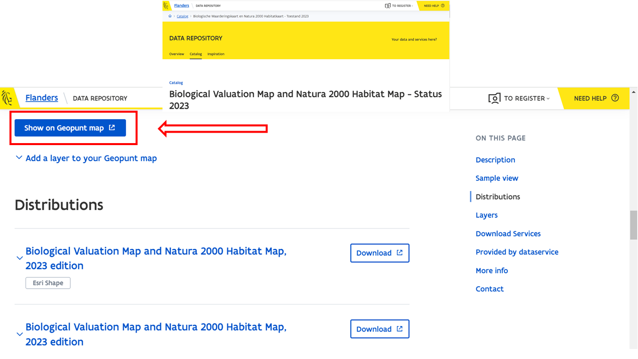
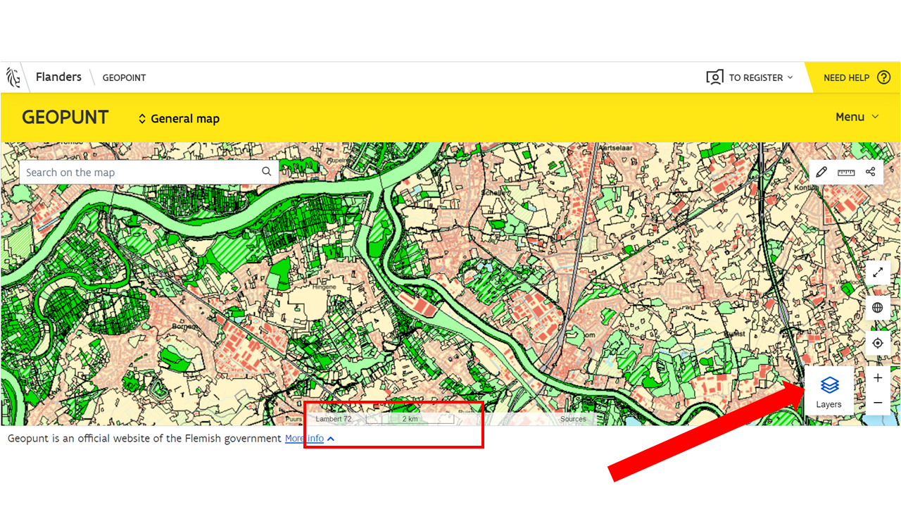
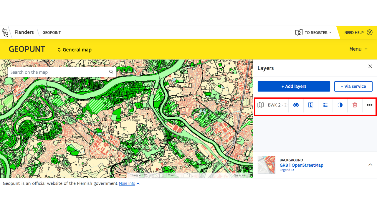
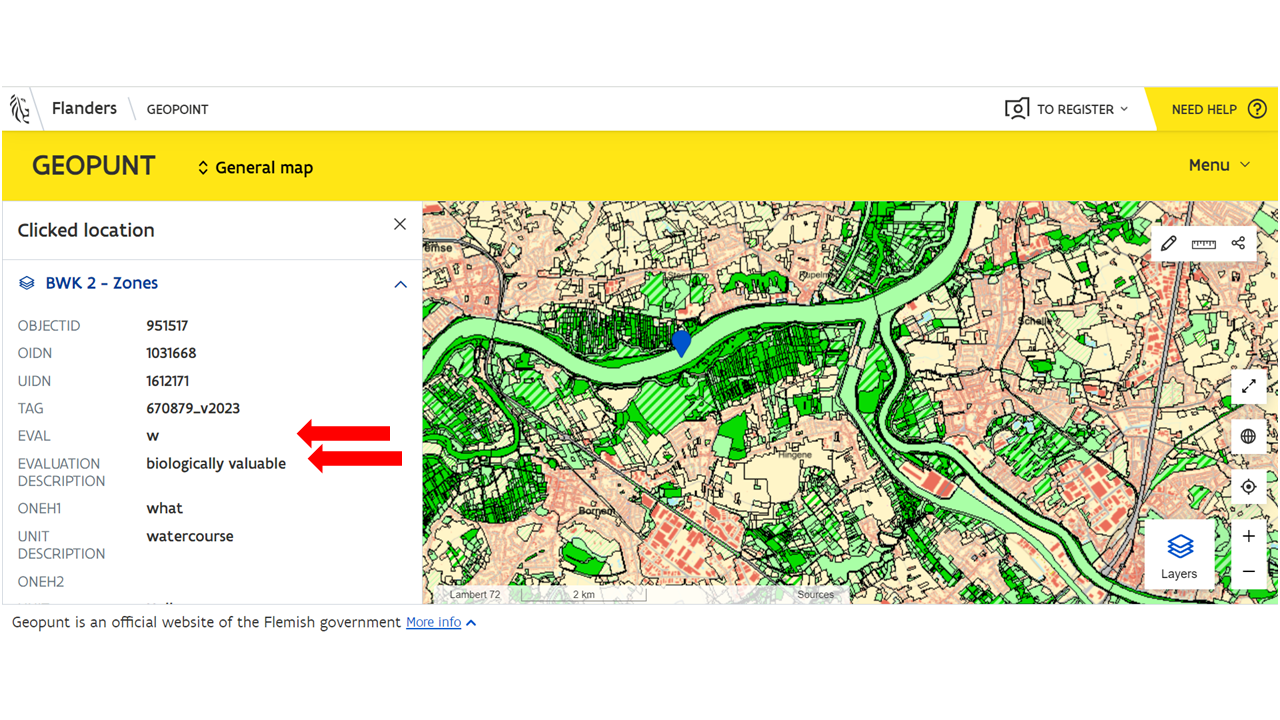
While this approach allows **basic exploration**, it does not enable **integration with EUNIS data**. To perform in-depth analysis, we need to **download the dataset** or use an **API endpoint** in GIS software.
Downloading the BWK Dataset
To manually download the dataset:
- Go to this metadata page.
- Click **"Download"** and export the files as a ZIP.
- Unzip the files. The dataset includes:
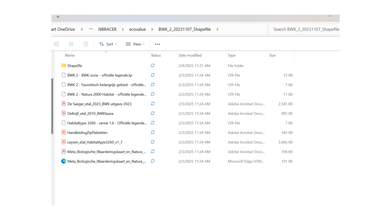
- BWK 2 Zone: Main ecological valuation dataset (Shapefile format).
- Habfauna & Hab3260: Additional datasets for biodiversity assessment.
- Metadata PDF: Important documentation about the dataset.
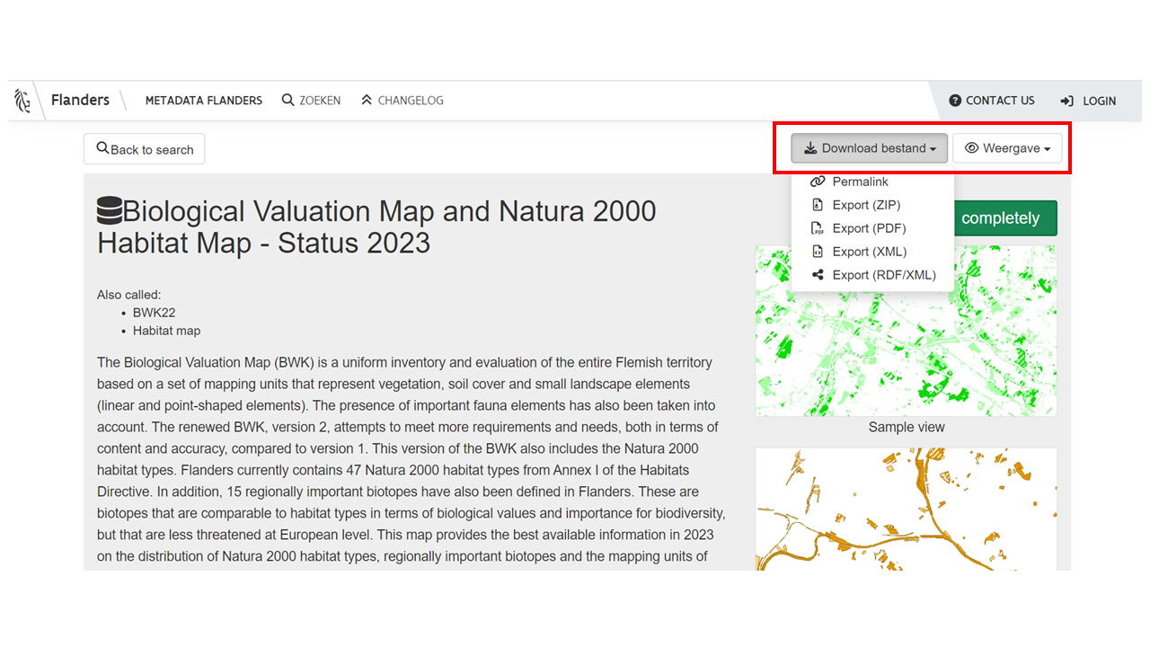
Before proceeding with GIS analysis, **review the metadata file** to understand the dataset structure.
Loading the Data into QGIS
To visualize the dataset in **QGIS**, follow these steps:
- Open **QGIS**.
- Go to **Layer → Add Vector Layer**.
- Navigate to the **BWK 2 Zone Shapefile** and click **Open**.
- To apply symbology, go to **Layer Properties → Symbology → Load Style**.
- Select the **.lyr or .sld file** included in the ZIP.
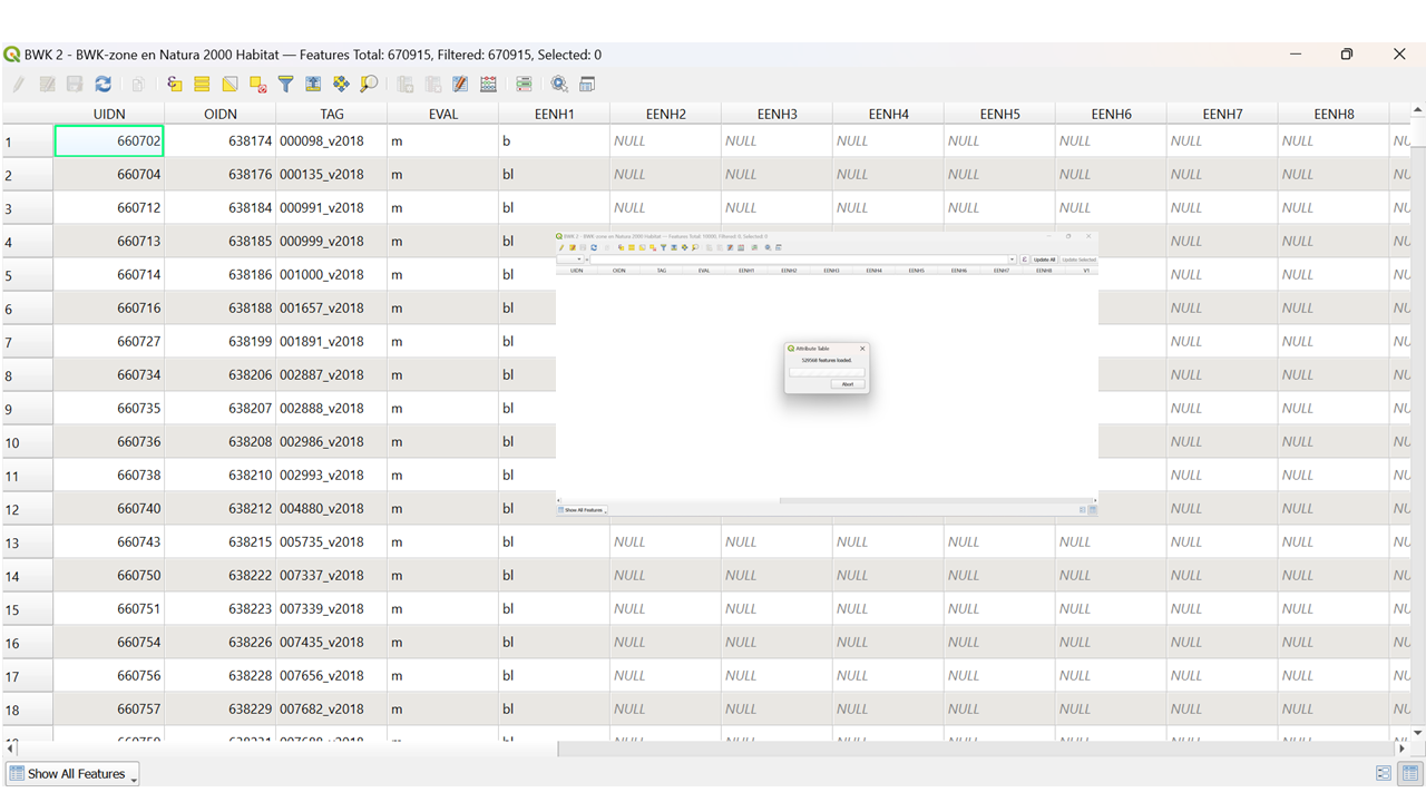
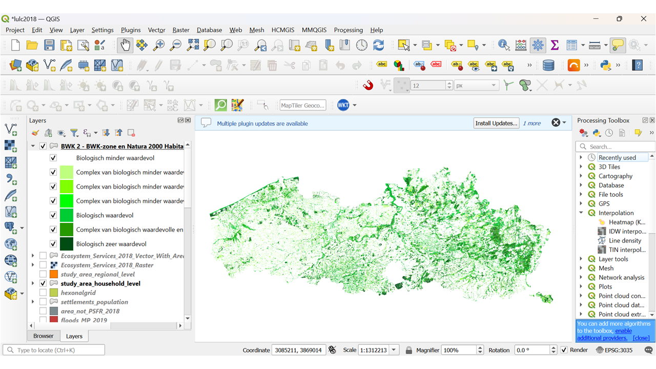
Loading the Data into ArcGIS Pro
To visualize the dataset in **ArcGIS Pro**, follow these steps:
- Open **ArcGIS Pro**.
- Click **Add Data** and browse to the **BWK 2 Zone Shapefile**.
- Drag and drop the layer onto the **Map panel**.
- Right-click the layer, select **Symbology**, and load the **LYR file**.
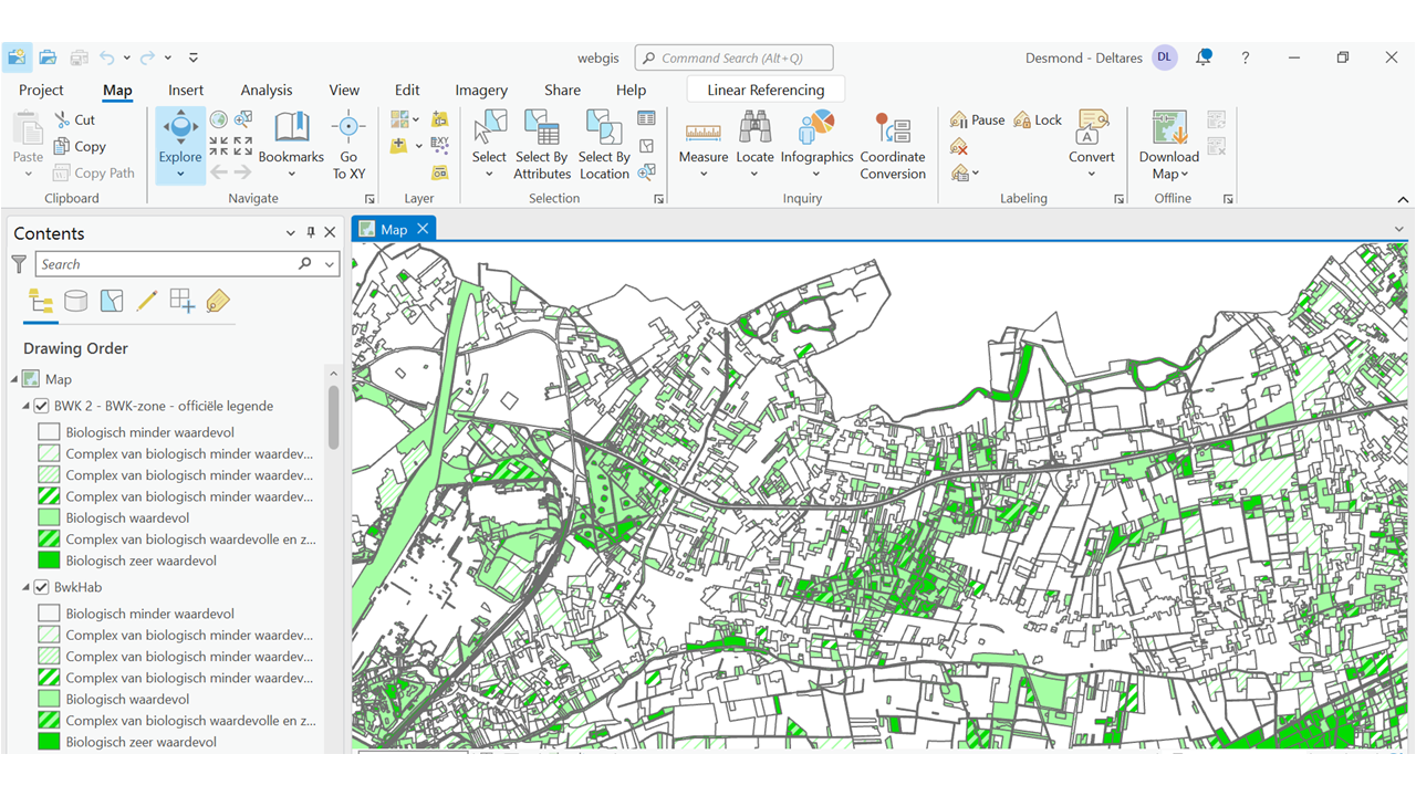
Screenshot Placeholder: ArcGIS Pro Symbology Setup
Accessing the Dataset via API (WFS/WMS)
Instead of downloading files, you can access the dataset via **API endpoints**:
- WMS Endpoint: Geopunt API.
- WFS Endpoint: Metadata API.
Steps to Load WMS/WFS in QGIS
- Go to **Layer → Data Source Manager → WMS/WMTS**.
- Click **"New"** and enter the **WMS API URL**.
- Load the layers and inspect attributes.
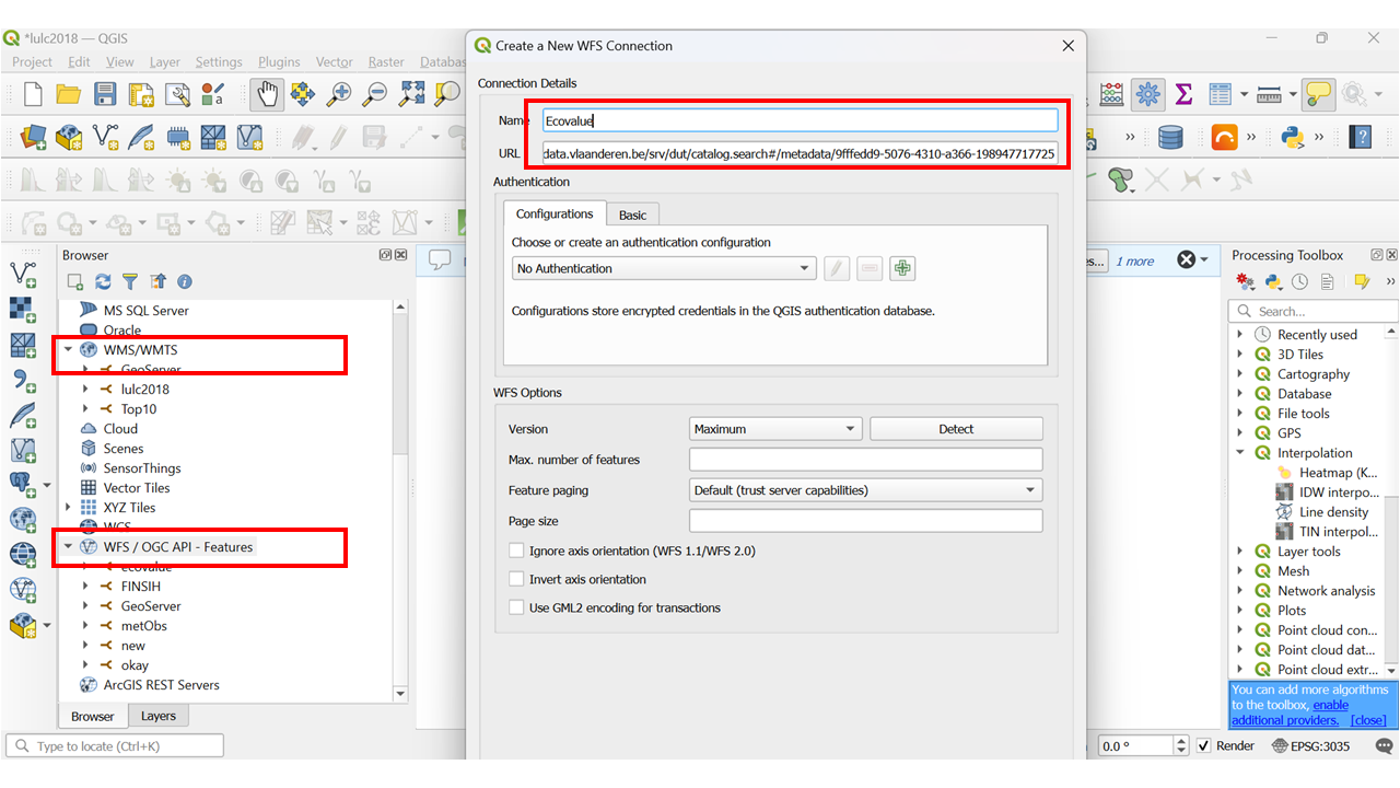
Steps to Load WMS/WFS in ArcGIS Pro
- Go to **Insert → Connections → Server → Add WMS Server**.
- Enter the **API endpoint** and add layers to the map.
Python Script for Automated Data Download
The dataset can also be downloaded programmatically using Python:
import requests
import geopandas as gpd

# API Endpoint for BWK Data
bwk_api_url = "https://metadata.vlaanderen.be/srv/dut/catalog.search#/metadata/9fffedd9-5076-4310-a366-198947717725"

# Download Data
response = requests.get(bwk_api_url)
if response.status_code == 200:
    with open("BWK_data.zip", "wb") as file:
        file.write(response.content)
    print("Download successful. Extract and load in QGIS/ArcGIS.")
else:
    print("Failed to download data.")
Integrating BWK Data with EUNIS Habitat Data
Now that we have loaded the dataset, the next step is to **integrate it with EUNIS habitat data**. If you downloaded the BWK dataset manually, it is in **vector format**, so ensure that the **EUNIS dataset** is also in the same format.
Spatial Join for Desktop GIS
The best method to merge both datasets in **QGIS or ArcGIS** is **spatial join**:
- Go to **Vector → Data Management Tools → Join Attributes by Location**.
- Select **EUNIS as the target layer** and **BWK as the join layer**.
- Choose **"intersects"** as the spatial operation.
- Export the result as a **new dataset**.
We do not cover this spatial operation in this guide since we want to do this in a cloud computing environment. If you want to do this you can consult other resources on how to perform a spatial join.
Cloud-Based Integration (Google Earth Engine)
Given the **large file size** (100,000+ polygons), **cloud processing** is preferable. We will **upload the BWK dataset to Earth Engine** and use it alongside the **EUNIS dataset stored as an asset**.
Step 1: Load Existing EUNIS & BWK Data
Before performing any spatial analysis, we need to **load the required datasets into Google Earth Engine (GEE)**. This includes:
- EUNIS Habitat Classification (Raster): A processed habitat dataset for the year 2018.
- BWK Ecological Valuation (Vector): A dataset containing **ecological quality ratings** for land units.
- Study Region (West Flanders, Belgium): The bounding box coordinates for our analysis.
Combining these datasets will allow us to assess the **ecological value of different EUNIS habitat types**. However, we first need to:
- Check that the **EUNIS raster contains the correct bands**.
- Inspect the **BWK vector attributes** before further processing.
- Define a **Region of Interest (ROI)** for analysis.
The following script loads the datasets and prints basic information for validation:
// Create a legend panel
// ===============================
// **LOAD EXISTING EUNIS & BWK DATA**
// ===============================

// Load the EUNIS habitat raster dataset (processed version)
var eunis = ee.Image("projects/ee-desmond/assets/EUNIS_2018_TIFF_nbracer");

// Load the BWK ecological valuation shapefile
var bwk = ee.FeatureCollection("projects/ee-desmond/assets/BwkHab");

// Define the region of interest (West Flanders, Belgium)
var region = ee.Geometry.BBox(2.5, 50.7, 4.0, 51.4);

// ===============================
// **DEBUGGING: PRINT AVAILABLE PROPERTIES & BANDS**
// ===============================

print(" EUNIS Image Properties:", eunis);
print("EUNIS Image Bands:", eunis.bandNames());  // Ensure correct band names
print(" BWK First Feature:", bwk.first());  // Inspect BWK structure
- The script **imports EUNIS** as a raster image and **BWK as a feature collection**.
- The study area is defined as a **bounding box (BBox)** for the West Flanders region.
- The **print() function** helps inspect the datasets to ensure correctness before proceeding.
Expected Output
When you run the script in **Google Earth Engine**, you should see:
- A **list of bands** available in the **EUNIS raster**.
- The **first feature** in the **BWK dataset**, showing its attribute fields.
- A **geometry object** defining the West Flanders region.
Next Step
Now that we have successfully loaded the datasets, the next step is to **convert BWK ecological categories into numeric values** so they can be used in geospatial calculations.
Step 2: Convert BWK 'EVAL' Property to Numeric Values
The **BWK dataset** contains an attribute named **EVAL**, which assigns qualitative ecological values to land areas. However, these values are stored as **categorical text**, which is not suitable for raster calculations or spatial analysis. We need to **map these categories to numerical values**.
- **Raster datasets require numeric values** for classification and analysis.
- **Mathematical operations (e.g., reclassification, merging) need numeric data types**.
- **Ensures compatibility** between the BWK (vector) and EUNIS (raster) datasets.
Ecological Value Mapping Scheme
We will **map the BWK categorical values to numerical equivalents** as follows:
| Categorical Value (EVAL) | Numerical Value (EVAL_NUM) | Ecological Meaning |
|---|---|---|
| z | 7 | Very High |
| wz | 6 | High |
| w | 5 | Moderate |
| mwz | 4 | Low-Moderate |
| mw | 3 | Low |
| m | 2 | Very Low |
| Missing / Undefined | 1 | Unknown |
The following script **applies the mapping function to the BWK dataset**:
// ===============================
// **STEP 2: CONVERT BWK 'EVAL' PROPERTY TO NUMERIC**
// ===============================

// Define mapping of categorical BWK values to numeric scores
var bwkCategoryToNumeric = {
'z': 7,  // Very High
'wz': 6, // High
'w': 5,  // Moderate
'mwz': 4, // Low-Moderate
'mw': 3,  // Low
'm': 2    // Very Low
};

// Function to apply the mapping to BWK features
var bwkNumeric = bwk.map(function(feature) {
var evalValue = feature.get('EVAL');  // Get categorical value
var numericValue = ee.Number(ee.Dictionary(bwkCategoryToNumeric).get(evalValue, 1)); // Default to 1 if missing
return feature.set('EVAL_NUM', numericValue);
});

// Debugging Print: Sample BWK Feature with Numeric Values
print("BWK First Feature with Numeric 'EVAL_NUM':", bwkNumeric.first());
- Dictionary Mapping (bwkCategoryToNumeric): - This object defines **how text-based values ('z', 'wz', etc.) map to numeric values (7, 6, etc.)**.
bwk.map(function(feature) {...}): - This function **iterates through each feature in the BWK dataset**, applying the numeric mapping.feature.get('EVAL'): - Retrieves the **existing categorical value** for each BWK feature.ee.Number(ee.Dictionary(bwkCategoryToNumeric).get(evalValue, 1)): - Converts the **text value into a number** using the dictionary. - If no match is found, it **assigns a default value of 1 (Unknown).**feature.set('EVAL_NUM', numericValue): - Adds the new **numeric attribute (EVAL_NUM)** to each feature.
After running the script, the **first feature in the BWK dataset** should now have a new property:
Feature {
geometry: (Polygon)
properties: {
    EVAL: "w",
    EVAL_NUM: 5  // Now in numeric format
}
}
Next Step
Now that the **BWK dataset has numeric values**, we can proceed to the next step: **Rasterizing BWK to match the EUNIS resolution**.
Step 3: Rasterizing BWK to Match EUNIS Resolution
The **BWK dataset** is currently in **vector format**, meaning it consists of **polygon geometries** representing different ecological valuation zones. However, to analyze this data alongside the **EUNIS habitat raster dataset**, we need to **convert BWK into a raster format**. This process is called **rasterization**.
Why Is Rasterization Important?
- **Raster data allows pixel-based spatial analysis**, making computations easier and faster.
- **Ensures compatibility with the EUNIS dataset**, which is already in raster format.
- **Reduces processing complexity** when performing operations like overlays and classifications.
The following script converts the **BWK ecological value polygons** into a raster, using the **EVAL_NUM field** (which we created in Step 2).
// ===============================
// **STEP 3: RASTERIZE BWK TO MATCH EUNIS RESOLUTION**
// ===============================

// Convert BWK features to raster using the 'EVAL_NUM' property
var bwkValues = bwkNumeric.reduceToImage({
  properties: ['EVAL_NUM'],
  reducer: ee.Reducer.first()  // Assigns first valid value per pixel
}).rename('ecological_value');

// Debugging Print: Rasterized BWK Values
print(" Rasterized BWK Values (ecological_value):", bwkValues);

// Align BWK raster to match EUNIS spatial resolution
bwkValues = bwkValues.reproject({
  crs: eunis.projection(),  // Use EUNIS coordinate reference system
  scale: eunis.projection().nominalScale()  // Match pixel size
});

print(" Reprojected BWK Raster:", bwkValues);
bwkNumeric.reduceToImage(): - Converts the **BWK vector polygons into a raster** using the **EVAL_NUM** field. - Uses **ee.Reducer.first()** to assign the first encountered value to each pixel..rename('ecological_value'): - Gives the new raster band a **meaningful name (ecological_value)**.bwkValues.reproject(): - Ensures the **BWK raster has the same coordinate reference system (CRS) and resolution as EUNIS**.eunis.projection(): - Retrieves the **projection system of the EUNIS dataset**, ensuring alignment.eunis.projection().nominalScale(): - Ensures the **BWK raster uses the same pixel size** as EUNIS.
Expected Output
After running the script, BWK should be successfully **converted into a raster**. The raster should now have an **ecological_value** band, where each pixel represents an ecological valuation score.
Raster Properties:
- Band Name: ecological_value
- Pixel Size: Matches EUNIS raster
- Projection: EPSG:4326
- Data Type: Integer (1-7)
Next Step
Now that the **BWK dataset is rasterized**, we can move to the next step: **Combining the BWK raster with the EUNIS habitat raster.**
Step 4: Exporting the BWK Dataset for Crosswalk Analysis
Now that we have **merged the EUNIS habitat dataset with BWK ecological values**, the next step is to **export the BWK dataset as a raster asset** in Google Earth Engine.
Why Do We Need to Export the BWK Dataset?
- 🔹 **Converting BWK from a feature collection to raster** ensures compatibility with raster-based analysis.
- 🔹 This raster will serve as the **foundation for crosswalk analysis**, where we compare **EUNIS habitat types** with **BWK ecological values**.
- 🔹 Exporting the dataset allows **efficient spatial sampling**, avoiding excessive processing load.
The following script exports the **BWK raster dataset** so that it can be later used for **sampling and crosswalk table generation**.
    // ===============================
    // **STEP 4: EXPORT BWK DATASET AS A RASTER**
    // ===============================

    // Export BWK dataset as a raster asset in Google Earth Engine
    Export.image.toAsset({
      image: eunisWithBwk,
      description: 'EUNIS_BWK_EcoValue_TIFF',
      assetId: 'projects/ee-desmond/assets/EUNIS_BWK_EcoValue_TIFF',
      region: region,
      scale: 100,
      crs: 'EPSG:4326',
      maxPixels: 1e13
    });
Export.image.toAsset(): - Saves the **BWK raster dataset** as an **Earth Engine asset** for later use.image: eunisWithBwk: - Specifies that we are exporting **EUNIS with BWK values merged**.region: region: - Defines the **study area (West Flanders, Belgium)**.scale: 100: - Ensures that the **raster resolution** is **100 meters per pixel**.crs: 'EPSG:4326': - Ensures a **consistent spatial reference system** (WGS84).maxPixels: 1e13: - Ensures the dataset can be processed without exceeding Earth Engine’s limits.
Expected Output
After running this export command, you should find the **EUNIS_BWK_EcoValue_TIFF** stored under **"Assets" in Google Earth Engine**.
projects/ee-desmond/assets/EUNIS_BWK_EcoValue_TIFF
Next Step: Performing the Crosswalk Analysis
With the **BWK dataset now available in raster format**, we can proceed to **Step 5**, where we will extract **random sample points** and generate a **crosswalk table** comparing **habitat types with ecological values**.
Step 5: Generating a Crosswalk Table
Now that we have the **EUNIS habitat** and **BWK ecological valuation** datasets stored as a raster asset, we can proceed with generating a **crosswalk table** that maps **habitat types to their ecological valuation**.
Why is a Crosswalk Table Important?
- Helps **quantify** the ecological value of different land cover types.
- Allows for **comparative analysis** of habitat resilience and biodiversity.
- Supports **nature-based solutions (NbS)** planning for climate adaptation.
- Provides structured data that can be used in **spatial modeling**.
The following script **samples raster values** at randomly generated locations and creates a **crosswalk table linking habitat types to their ecological value**.
// ===============================
// **STEP 5: CROSSWALK TABLE GENERATION**
// ===============================

//  Load the updated raster dataset with EUNIS + BWK data
var eunisWithBwkUpdated = ee.Image("projects/ee-desmond/assets/EUNIS_BWK_EcoValue_TIFF");
print(" Loaded Final Raster for Crosswalk Table Generation:", eunisWithBwkUpdated);

//  Extract EUNIS and Ecological Value bands
var eunisBand = eunisWithBwkUpdated.select('eunis');
var ecoValueBand = eunisWithBwkUpdated.select('ecological_group');
print(" EUNIS Band:", eunisBand);
print(" Ecological Value Band:", ecoValueBand);

//  Generate Random Sample Points within the Study Region
var samplePoints = ee.FeatureCollection.randomPoints({
region: region,
points: 5000, // Limit to avoid exceeding feature count
seed: 42
});
print(" Generated Sample Points:", samplePoints);

//  Extract EUNIS and Ecological Values at Sampled Locations
var sampledValues = eunisWithBwkUpdated.sampleRegions({
collection: samplePoints,
scale: 100,
properties: [],
tileScale: 4  // Optimized for large collections
});
print(" Sampled Raster Values:", sampledValues.limit(10)); // Preview first 10 rows

//  Convert Sampled Data into a Feature Collection Table
var eunisMapping = ee.Dictionary(eunisNumericMapping); // Convert to EE dictionary

var crosswalkTable = sampledValues.map(function(feature) {
var eunisClass = feature.get('eunis');  // Extract EUNIS class ID
var ecoValue = feature.get('ecological_group'); // Extract Ecological Value

// Convert EUNIS class to a string key for dictionary lookup
var eunisKey = ee.Algorithms.If(eunisClass, ee.String(eunisClass), 'Unknown');

// Ensure the key exists in the dictionary, else assign default values
var hasKey = eunisMapping.contains(eunisKey);

var eunisEntry = ee.Algorithms.If(
hasKey,
eunisMapping.get(eunisKey),
ee.Dictionary({'eunisCode': 'Unknown', 'description': 'Unknown Habitat', 'color': '#808080'})
);

var eunisCode = ee.String(ee.Dictionary(eunisEntry).get('eunisCode'));
var eunisDesc = ee.String(ee.Dictionary(eunisEntry).get('description'));
var eunisColor = ee.String(ee.Dictionary(eunisEntry).get('color'));

return feature.set({
'EUNIS Code': eunisCode,
'EUNIS Habitat': eunisDesc,
'EUNIS Color': eunisColor,
'Ecological Value': ecoValue
});
});

//  Convert to Feature Collection for Table View
var crosswalkFC = ee.FeatureCollection(crosswalkTable);
print(" Final Crosswalk Table (Sampled Pixels):", crosswalkFC.limit(10)); // Preview first 10 rows

//  Export as a CSV for non-GIS users
Export.table.toDrive({
collection: crosswalkFC,
description: 'EUNIS_Ecological_Crosswalk_Sampled',
fileFormat: 'CSV'
});
print(" Export Task Created: Run it manually in the 'Tasks' tab!");
sampleRegions(): - Extracts **EUNIS habitat type** and **BWK ecological value** at **random points**.randomPoints(): - Generates **5000 random sample locations** across the study area.map(): - Iterates through each sampled location, **retrieving habitat and ecological value**.Export.table.toDrive(): - Exports the **final crosswalk table** as a **CSV file**.
Expected Output
After running this script, you will find a **crosswalk table** available in Google Drive as a **CSV file**, which links:
EUNIS Habitat Type → BWK Ecological Value
----------------------------------------
Forest (T1)        → Very High (7)
Urban Area (J1)    → Low (2)
Wetland (C1)       → High (6)
Next Step: Visualizing the Data
With the **crosswalk table completed**, we will move to **Step 6**, where we visualize the dataset and interpret key insights from the analysis on the map canvas.
Step 6: Map Visualization
With the **crosswalk table** completed, we can now visualize the EUNIS habitat types and BWK ecological valuation data in Google Earth Engine.
- Helps **identify spatial patterns** in ecological value.
- Supports **policy-making and conservation planning**.
- Allows for **interactive exploration of habitat quality**.
The following script **renders an interactive map** with a **legend showing ecological value classifications**.
// ===============================
// **STEP 6: MAP VISUALIZATION**
// ===============================

var eunisNumericMapping = {
  1: {eunisCode: 'J1', color: '#b22222', description: 'Buildings of cities, towns, and villages'},
  2: {eunisCode: 'J1.2', color: '#ff4500', description: 'Residential buildings of villages and urban peripheries'},
  3: {eunisCode: 'J2', color: '#ffa07a', description: 'Low density buildings'},
  4: {eunisCode: 'J4', color: '#8b4513', description: 'Transport networks and other hard-surfaced areas'},
  5: {eunisCode: 'J4.5', color: '#d2691e', description: 'Hard-surfaced areas of ports'},
  6: {eunisCode: 'J4.4', color: '#808080', description: 'Airport runways and aprons'},
  7: {eunisCode: 'J3', color: '#556b2f', description: 'Extractive industrial sites'},
  8: {eunisCode: 'J6', color: '#a0522d', description: 'Waste deposits'},
  9: {eunisCode: 'J1.6', color: '#d2b48c', description: 'Urban and suburban construction and demolition sites'},
  10: {eunisCode: 'X11-2012', color: '#deb887', description: 'Large parks'},
  1: {eunisCode: 'J1-2012', color: '#b22222', description: 'Buildings of cities, towns, and villages'},
  11: {eunisCode: 'V1', color: '#32cd32', description: 'Arable land and market gardens'},
  12: {eunisCode: 'V11', color: '#adff2f', description: 'Intensive unmixed crops'},
  13: {eunisCode: 'V14', color: '#ff7f50', description: 'Inundated or inundatable croplands, including rice fields'},
  14: {eunisCode: 'V54', color: '#8fbc8f', description: 'Vineyards'},
  15: {eunisCode: 'V53', color: '#228b22', description: 'Shrub plantations for ornamental purposes or for fruit, other than vineyards'},
  16: {eunisCode: 'T24', color: '#f4a460', description: 'Olea europaea-Ceratonia siliqua woodland'},
  17: {eunisCode: 'R2', color: '#006400', description: 'Mesic grasslands'},
  18: {eunisCode: 'V1', color: '#ffe4b5', description: 'Arable land and market gardens'},
  19: {eunisCode: 'V2', color: '#6b8e23', description: 'Cultivated areas of gardens and parks'},
  20: {eunisCode: 'V13', color: '#f0e68c', description: 'Arable land with unmixed crops grown by low-intensity agricultural methods'},
  21: {eunisCode: 'R7', color: '#d2b48c', description: 'Sparsely wooded grasslands'},
  22: {eunisCode: 'T1', color: '#008000', description: 'Broadleaved deciduous woodland'},
  23: {eunisCode: 'T3', color: '#3cb371', description: 'Coniferous woodland'},
  24: {eunisCode: 'G4-2012', color: '#20b2aa', description: 'Mixed deciduous and coniferous woodland'},
  25: {eunisCode: 'R1', color: '#7cfc00', description: 'Dry grasslands'},
  26: {eunisCode: 'S4', color: '#8b0000', description: 'Temperate shrub heathland'},
  27: {eunisCode: 'F5', color: '#b0c4de', description: 'Maquis, arborescent matorral, and thermo-Mediterranean brushes'},
  28: {eunisCode: 'R5', color: '#87cefa', description: 'Woodland fringes and clearings and tall forb stands'},
  29: {eunisCode: 'N1', color: '#fa8072', description: 'Coastal dunes and sandy shores'},
  30: {eunisCode: 'MA1', color: '#add8e6', description: 'Littoral rock and other hard substrata'},
  31: {eunisCode: 'U5', color: '#708090', description: 'Miscellaneous inland habitats with very sparse or no vegetation'},
  32: {eunisCode: 'H5.5-2012', color: '#d3d3d3', description: 'Burnt areas with very sparse or no vegetation'},
  33: {eunisCode: 'U4', color: '#556b2f', description: 'Snow or ice-dominated habitats'},
  34: {eunisCode: 'C3-2012', color: '#4169e1', description: 'Littoral zone of inland surface waterbodies'},
  35: {eunisCode: 'D1-2012', color: '#00bfff', description: 'Raised and blanket bogs'},
  36: {eunisCode: 'A2.5', color: '#1e90ff', description: 'Coastal saltmarshes and saline reedbeds'},
  37: {eunisCode: 'J5.1-2012', color: '#6495ed', description: 'Highly artificial saline and brackish waters'},
  38: {eunisCode: 'MA5', color: '#ffdab9', description: 'Littoral sand'},
  39: {eunisCode: 'C2-2012', color: '#87ceeb', description: 'Surface running waters'},
  40: {eunisCode: 'C1-2012', color: '#2171b5', description: 'Surface standing waters'},
  41: {eunisCode: 'X02-2012', color: '#ffdab9', description: 'Saline coastal lagoons'},
  42: {eunisCode: 'X01-2012', color: '#2171b5', description: 'Estuaries'},
  43: {eunisCode: 'MB5', color: '#87cefa', description: 'Infralittoral sand'}
};


// Define visualization parameters for EUNIS habitats
var eunisVisParams = {
  min: 1,
  max: 44,
  palette: Object.keys(eunisNumericMapping).map(function(key) {
    return eunisNumericMapping[key].color;
  })
};

// Print available bands in the final raster before visualization
print(" Final Raster Bands:", eunisWithBwk.bandNames());

// Define visualization parameters for the 7-group classification
var visParams = {
  min: 2,  // Change from 1 to 2
  max: 7,
  palette: ['#edf8fb', '#ccece6', '#99d8c9', '#66c2a4', '#41ae76', '#238b45'] // Correct order
};


// Load the processed EUNIS raster with ecological values
var eunisEcoValue = ee.Image("projects/ee-desmond/assets/EUNIS_BWK_EcoValue_TIFF");
print(" Loaded Final Raster for Visualization:", eunisEcoValue);

// Center the map on the study region
Map.centerObject(region, 10);

// Add the ecological classification layer
Map.addLayer(eunisEcoValue.select('ecological_group'), visParams, "Ecological Value Classification");

// **🔹 Add the Legend**
var legend = ui.Panel({
  style: {
    position: 'bottom-left',
    padding: '8px',
    backgroundColor: 'white'
  }
});

// Add title to the legend
legend.add(ui.Label({
  value: 'Ecological Value Classification',
  style: { fontWeight: 'bold' }
}));

// Correct classification labels matching raster values (2 to 7)
var labels = ['Very Low', 'Low', 'Low-Moderate', 'Moderate', 'High', 'Very High'];
var colors = ['#edf8fb', '#ccece6', '#99d8c9', '#66c2a4', '#41ae76', '#238b45'];  // Matches visParams

// Clear previous legend (if any)
var legend = ui.Panel({
  style: {
    position: 'bottom-left',
    padding: '8px',
    backgroundColor: 'white'
  }
});

// Add title
legend.add(ui.Label({
  value: 'Ecological Value Classification',
  style: { fontWeight: 'bold' }
}));

// Add legend entries dynamically (matching raster values)
labels.forEach(function(label, index) {
  legend.add(ui.Panel([
    ui.Label({
      style: {
        backgroundColor: colors[index],
        padding: '8px',
        margin: '0px 4px 4px 0',
        border: '1px solid black'
      }
    }),
    ui.Label({
      value: label,
      style: { margin: '0px 0px 4px 6px' }
    })
  ], ui.Panel.Layout.Flow('horizontal')));
});

// Add the corrected legend to the map
Map.add(legend);
print(" Legend updated and added to the map.");

// Add EUNIS habitat map to the display
Map.centerObject(region, 10);
Map.addLayer(eunis, eunisVisParams, "EUNIS Habitat Classification");
Map.addLayer(): - Displays the **ecological valuation layer** on the map.ui.Panel(): - Creates an **interactive legend** for visualization.palette: - Assigns **colors** to different ecological value classes.
Expected Output
After running this script, the map will display:
- **EUNIS habitat classifications** (colored by land cover type).
- **BWK ecological valuation classes** (ranging from very high to very low).
- **An interactive legend** showing the color scheme for each category.
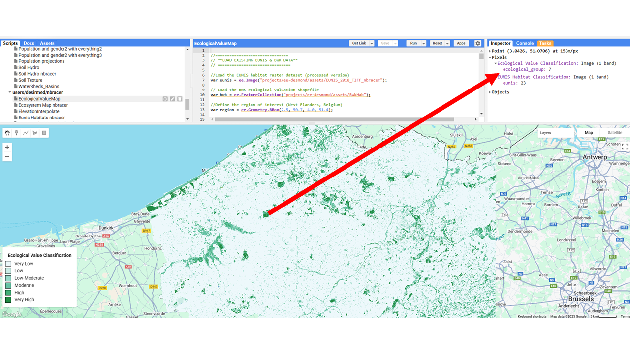
We can now better understand how different habitats contribute to resilience, biodiversity, and nature-based solutions based on their ecological value.