Climate Risk Impact Chain Assessment

workflowr

• Summary
• Checks
• Past versions

Last updated: 2025-01-02

Checks: 7 0

Knit directory: nbs-workflow/

This reproducible R Markdown analysis was created with workflowr (version 1.7.1). The Checks tab describes the reproducibility checks that were applied when the results were created. The Past versions tab lists the development history.

---

R Markdown file: up-to-date

Great! Since the R Markdown file has been committed to the Git repository, you know the exact version of the code that produced these results.

Environment: empty

Great job! The global environment was empty. Objects defined in the global environment can affect the analysis in your R Markdown file in unknown ways. For reproduciblity it’s best to always run the code in an empty environment.

Seed: set.seed(20241223)

The command set.seed(20241223) was run prior to running the code in the R Markdown file. Setting a seed ensures that any results that rely on randomness, e.g. subsampling or permutations, are reproducible.

Session information: recorded

Great job! Recording the operating system, R version, and package versions is critical for reproducibility.

Cache: none

Nice! There were no cached chunks for this analysis, so you can be confident that you successfully produced the results during this run.

File paths: relative

Great job! Using relative paths to the files within your workflowr project makes it easier to run your code on other machines.

Repository version: 08ce7da

Great! You are using Git for version control. Tracking code development and connecting the code version to the results is critical for reproducibility.

The results in this page were generated with repository version 08ce7da. See the Past versions tab to see a history of the changes made to the R Markdown and HTML files.

Note that you need to be careful to ensure that all relevant files for the analysis have been committed to Git prior to generating the results (you can use wflow_publish or wflow_git_commit). workflowr only checks the R Markdown file, but you know if there are other scripts or data files that it depends on. Below is the status of the Git repository when the results were generated:

Ignored files:
    Ignored:    .Rhistory
    Ignored:    .Rproj.user/

Untracked files:
    Untracked:  data/raster/reclassified.tif
    Untracked:  data/raster/reclassified.tif.aux.xml

Note that any generated files, e.g. HTML, png, CSS, etc., are not included in this status report because it is ok for generated content to have uncommitted changes.

---

These are the previous versions of the repository in which changes were made to the R Markdown (analysis/Climate Risk Impact Chain Assessment.Rmd) and HTML (docs/Climate Risk Impact Chain Assessment.html) files. If you’ve configured a remote Git repository (see ?wflow_git_remote), click on the hyperlinks in the table below to view the files as they were in that past version.

File	Version	Author	Date	Message
Rmd	08ce7da	Desmond Lartey	2025-01-02	wflow_publish("analysis/Climate Risk Impact Chain Assessment.Rmd")
html	f631618	Desmond Lartey	2025-12-31	Build site.
html	a7faec7	Desmond Lartey	2025-02-28	Build site.
Rmd	777eca0	Desmond Lartey	2025-02-28	wflow_publish("analysis/Climate Risk Impact Chain Assessment.Rmd")
html	7d70ba7	Desmond Lartey	2025-02-28	Build site.
Rmd	6c19bd7	Desmond Lartey	2025-02-28	wflow_publish("analysis/Climate Risk Impact Chain Assessment.Rmd")

---

Understanding Landscape Characterization in DesirMED

You remeber that In Task 4.1, we went through the process of systematically characterizing landscapes into the 3 domains i.e biophysical, socio-economic, and governance. But why do this? Here, we will try to show you how T4.1 could be useful by linking these insights to broader climate resilience-building efforts. Because on the one hand you want to understandd your systems and its components, and on the hand, you want to see how the systems are interelated, services provision, how they are linked to the various risks and how these enhance our understanding of what climate adaptation solutions are necessary.

More specifically:

• How do we ensure that landscapes are not just viewed as static entities, but rather as dynamic systems with interdependent ecological, socio-economic, and governance structures?
• Can we use this characterization approach we adopted to identify patterns, vulnerabilities, and opportunities for intervention in climate adaptation strategies?
• What insights can we extract from this LAs to better support the development and implementation of Nature-based Solutions (NbS) at different scales?

At its core, landscape characterization allows us to go beyond mere classification. It provides a structured approach to:

• Identify and classify distinct landscape archetypes based on three key domains:
• Biophysical and Ecological Characteristics (e.g., terrain, vegetation, land cover, land use).
• Socio-Economic Dimensions (e.g., key community systems, infrastructure, economic activities).
• Governance (e.g., what structures are there to support climate resilient and adaptation srategies).

Linking Landscape Characterization to Climate Risk Impact Chain Assessment

A fundamental value of the approach we have used lies in its strong connection to climate risk impact chain assessment. By combining landscape characterization with impact chains, we can:

• Map out interrelations and cascading impacts between the various landscape domains, environmental hazards, risk exposure, vulnerabilities, and resilience capacity.
• Support the cross-linking of ecosystem services with socio-economic and governance structures, ensuring that existing natural systems are leveraged for risk reduction and sustainable development.
• Create an evidence-based foundation for NbS implementation and upscaling across different landscapes.
• Assess how existing ecosystem services (solutions) support resilience and mitigate cascading risks.
• Identify which community systems are at risk and which NbS interventions have the potential to mitigate this risk(s) and address regional needs for increased climate resilience.
• Provide a structured approach to guide decision-making in spatial planning, policy, and investment for resilience-building.

This interrelatedness also allows us to critically assess our system—not in isolation but in its complexity. It moves us beyond fragmented analysis and enables a more holistic assessment of our socio-ecological landscape systems.

How Should the Final Product Look?

While the draft product concept provides a structured approach, we acknowledge that this is not set in stone. The methodology must evolve as we integrate expert input and stakeholder feedback. To ensure practical usability, we are exploring different final product formats, including:

• A Structured Overarching Table – A matrix summarizing key landscape archetypes, their risks, ecosystem services, and NbS opportunities for decision-makers to guide portfolio development and upscaling strategies. We expect this output to be landscape-specific and not general/generic
• An Interactive Media Documentation – A more descriptive and qualitative approach, combining maps, narratives, and stakeholder feedback to create a visually rich and decision-supporting product. We also expect this to be specific per case area

We invite discussions on the approach and the final product. Could this methodology enhance our ability to assess and manage landscapes more effectively? How might we refine it further to maximize its impact on NbS portfolio development and upscaling?

Step-by-Step Integration of Landscape Characterization outputs with Risk Layers

Now, we will systematically integrate our landscape characterization outputs we created in the previous session with additional datasets for the impact chain. We will add datasets such as:

• Population Distribution (to assess demographic vulnerabilities and dependencies. This can be enriched with more socioeconomic factors such as critical infrastructures, economic hubs, tourism hubs, etc).
• EUNIS Habitat Data (to understand the ecological structure and services available in different regions).
• Ecosystems services (to understand the the services that are already being produced in each of these areas and their respective archetypes. How they are affected and they contribute to resilience).
• Flood Risk Scenarios (to analyze differential exposure across landscape archetypes, demographics, and socio-economic).

By layering these datasets, we will explore their interrelations, identify gaps, and refine our assessment of resilience and risk reduction opportunities. This step-by-step integration will provide a clearer picture of how different landscapes characters respond to hazards and how we can optimize NbS interventions

Let’s now proceed to show an example analysis of what we can make from the outputs of T4.1 (Landscape Characterisation).

You can view this presentation file for a better simple overview and scientific literature techniques adopted. You should NOT download this file because it content will always be improved with time.

ℹ️ Note: The richness of this impact chain assessment largely depends on the quality of datasets available for the region we used for the Landscape Characterisation exercise, especially on socio-economic and governance aspects. We do not expect biophysical factors to change in mapping.

To show what we can make from Taks 4.1, we will adopt the framework proposed in NBRACER

Step 1: Define the Spatial and Temporal Context

We utilize high-resolution geospatial datasets, including population demographics, landscape archetypes, ecosystem maps, and flood probabilities. This step establishes the geographic scope (landscape archetypes, regions) and assesses the interrelationship between climatic, ecological, and socio-economic factors shaping risk dynamics.

Step 2: Determine Hazards and Intermediate Impacts

We identify primary climate hazards such as flooding and extreme weather events. The spatial propagation of these hazards across biophysical and infrastructure systems is analyzed to understand their impact and where NbS interventions can be most effective.

Step 3: Determine Exposed Elements of the Socio-Ecological and Governance System

We identify Key Critical Sectors (KCS) at risk, including:

• Natural ecosystems (e.g., wetlands, forests)
• Infrastructure (e.g., roads, water supply, hospitals, urban areas). Note that we mainly use the POI datasets available to use. Check the process in the landscape characterization exercise
• Vulnerability and exposure (e.g., per communities, age and sex, population in different years)

Step 4: Determine Vulnerability of the Socio-Ecological System

We analyze how risks are associated with different landscape archetypes and evaluate social vulnerabilities by clustering indicators and identifying governance gaps. Risks are also analyzed in relation to governance and social-economic vulnerabilities, recognizing their interdependency.

Step 5: Conduct Spatial Analysis and Quantify Risk

We perform statistical summaries and intersection analysis to quantify risk levels across different regions and sectors. Existing ecosystem services are assessed to determine their contributions to resilience, and priority areas for NbS interventions are identified based on ecosystem functionality and exposure.

Step 6: Plan Responses and NbS-Based Adaptations

The final step involves generating key analysis outputs, including flood exposure assessments, resilience scores, and ecosystem contributions. We can then design NbS interventions targeted at mitigating climate risks, integrate governance frameworks for scalability, and establish monitoring mechanisms to track adaptation outcomes.

Step 1: Load Required Datasets

Before conducting any analysis, we need to load the necessary datasets in GEE.

• Settlement Data: Contains population and demographic information.
• Flood Probability Raster Data: Represents flood hazard probability at different levels.
• Ecosystem Services Data: Provides information on environmental functions.
• EUNIS Habitat Classification: A habitat classification system used for land cover analysis.
• Landscape Archetypes: Defines land character types based on morphology, vegetation, and land use.
• Point of Interest (POI) Data: Captures socio-economic infrastructure and service locations.

    // Load required datasets in GEE
    var settlements = ee.FeatureCollection("projects/ee-desmond/assets/desirmed/settlements_population_with_gender_age");
    var floodsHPRaster = ee.Image("projects/ee-desmond/assets/desirmed/floods_High_Probability_Raster");
    var floodsLPRaster = ee.Image("projects/ee-desmond/assets/desirmed/floods_Low_Probability_Raster");
    var floodsMPRaster = ee.Image("projects/ee-desmond/assets/desirmed/floods_Medium_Probability_Raster");
    var ecosystemServices = ee.Image("projects/ee-desmond/assets/desirmed/Ecosystem_Services_2018_Raster_Asset");
    var eunis = ee.Image("projects/ee-desmond/assets/desirmed/EUNIS_2018_TIFF");
    var archetypes = ee.Image("projects/ee-desmond/assets/desirmed/Archetype_2018_TIF");
    var poiDataset = ee.FeatureCollection('projects/ee-desmond/assets/desirmed/PointOfinterest');
    

Note

You can see that some of the datasets we are using for the impact chain assessment are new. These are already geoprocessed datasets which we dont cover how to make them in the workflow but we have made them all publicly available for you to use for this workshop.

• Ensure that all relevant datasets are loaded for analysis.
• We can then overlay multiple spatial datasets.
• Identify potential exposure and risk patterns.

Step 2: Calculate Flood Exposure for Each Settlement

Now that we have the required datasets, we will calculate the flood exposure for each settlement. This involves:

• Overlaying flood hazard rasters with the settlement boundaries.
• Computing the total area affected by floods.
• Storing the flood exposure values as attributes for further analysis.

    // Function to compute flood exposure for settlements
    function calculateFloodExposure(feature, floodRaster, floodType) {
        var floodArea = floodRaster.reduceRegion({
            reducer: ee.Reducer.sum(),
            geometry: feature.geometry(),
            scale: 30,
            maxPixels: 1e13
        }).get('first'); // Adjust band name if necessary
    
        floodArea = ee.Number(floodArea || 0).multiply(900).divide(1e6); // Convert pixels to km²
        return feature.set(floodType, floodArea);
    }
    
    // Apply function to settlements
    var settlementsWithFloodMetrics = settlements.map(function(feature) {
        feature = calculateFloodExposure(feature, floodsHPRaster, 'Flood_HP_Area_km2');
        feature = calculateFloodExposure(feature, floodsMPRaster, 'Flood_MP_Area_km2');
        feature = calculateFloodExposure(feature, floodsLPRaster, 'Flood_LP_Area_km2');
        return feature;
    });
    

• We use reduceRegion() to sum the flooded area within a settlement boundary.
• The result is converted into square kilometers (km²) for better interpretation.
• We apply this function to all three flood scenarios (high, medium, and low probability).

Next Steps

• We will now analyze ecosystem services within flood-prone settlements.
• Calculate resilience scores based on ecosystem coverage and exposure.
• Use visualization techniques to map and interpret the results.

➡ Next: Analyzing Ecosystem Services & Mapping Resilience

Step 3: Analyzing Ecosystem Services

Now that we have calculated flood exposure, we will analyze ecosystem services within these flood-prone areas. Understanding ecosystem services is crucial because:

• They act as natural flood buffers (e.g., wetlands absorb excess water).
• They contribute to climate adaptation by reducing vulnerabilities.
• They help in designing Nature-based Solutions (NbS) for flood risk management.

Extracting Ecosystem Services for Settlements

To compute the total ecosystem service contribution, we will:

• Extract ecosystem service values for each settlement.
• Aggregate different ecosystem service areas within a region.
• Calculate the proportion of each ecosystem service class.

      // Define ecosystem classes and their names
      var ecosystemClasses = [
        21100, 22100, 23100, 31100, 32100, 33100, 42100, 42200,
        51000, 71100, 71220, 72100, 81100, 82100
      ];
      
      var ecosystemServiceNames = {
        21100: 'Arable Land',
        22100: 'Vineyards & Orchards',
        23100: 'Annual Crops',
        31100: 'Broadleaved Forest',
        32100: 'Coniferous Forest',
        33100: 'Mixed Forest',
        42100: 'Semi-Natural Grassland',
        42200: 'Alpine Grassland',
        51000: 'Heathland',
        71100: 'Inland Marshes',
        71220: 'Peat Bogs',
        72100: 'Salt Marshes',
        81100: 'Natural Water Courses',
        82100: 'Natural Lakes'
      };

     // Function to compute ecosystem service contribution for each settlement
  function calculateEcosystemMetrics(feature) {
    var classAreas = ecosystemClasses.reduce(function(dict, classValue) {
      var classArea = ecosystemServices.eq(classValue).reduceRegion({
        reducer: ee.Reducer.sum(),
        geometry: feature.geometry(),
        scale: 30,
        maxPixels: 1e13
      }).get('remapped'); // Ensure the band name matches

      classArea = ee.Number(classArea || 0).multiply(900).divide(1e6); // Convert pixels to km²
      return dict.set(classValue.toString(), classArea);
    }, ee.Dictionary({}));

    // Calculate total ecosystem area
    var totalEcosystemArea = ee.Number(
      classAreas.values().reduce(ee.Reducer.sum()) // Sum of all ecosystem areas
    );

    // Calculate percentages for each class
    var classPercentages = classAreas.map(function(key, value) {
      return ee.Number(value).divide(totalEcosystemArea).multiply(100);
    });

    return feature.set('Ecosystem_Class_Areas', classAreas)
                  .set('Total_Ecosystem_Area_km2', totalEcosystemArea)
                  .set('Ecosystem_Class_Percentages', classPercentages);
  }

  var settlementsWithEcosystemMetrics = settlementsWithFloodMetrics.map(calculateEcosystemMetrics);

  print(settlementsWithEcosystemMetrics)
    

• reduceRegion() extracts specific ecosystem service values for each settlement.
• map() applies this function to all settlements in the dataset.
• Ecosystem_Class_Percentages helps in comparing settlements based on their ecosystem support.

Next: We will proceed with Resilience Scoring and Risk Categorization.

Step 4: Resilience Scoring & Risk Categorization

Now that we have both flood exposure and ecosystem service metrics, we will compute a Resilience Score to evaluate the ability of each settlement to cope with floods.

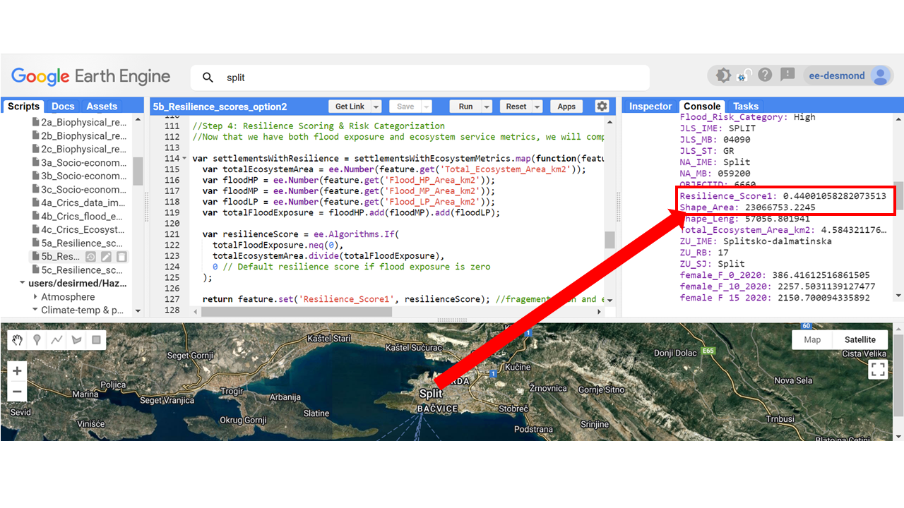
Compute a Resilience Score - option 1?

Methodology

The resilience score for Option 1 is computed using the following formula:

    Resilience Score = Total_Ecosystem_Area / ∑(Flood_HP_Area + Flood_MP_Area + Flood_LP_Area)
    

Where:

• Total_Ecosystem_Area: The total area (km²) covered by ecosystem services in the settlement.
• Flood_HP_Area: The area (km²) exposed to high-probability flooding.
• Flood_MP_Area: The area (km²) exposed to medium-probability flooding.
• Flood_LP_Area: The area (km²) exposed to low-probability flooding.
• ∑ (Sum): Indicates that we sum the flood exposure values across different probability levels.

This formula evaluates how much ecological space is available to mitigate flood exposure. A higher resilience score suggests that the settlement has more ecosystem services available relative to its flood exposure, which improves flood resilience.

    // Function to compute resilience score
    var settlementsWithResilience = settlementsWithEcosystemMetrics.map(function(feature) {
      var totalEcosystemArea = ee.Number(feature.get('Total_Ecosystem_Area_km2'));
      var floodHP = ee.Number(feature.get('Flood_HP_Area_km2'));
      var floodMP = ee.Number(feature.get('Flood_MP_Area_km2'));
      var floodLP = ee.Number(feature.get('Flood_LP_Area_km2'));
      var totalFloodExposure = floodHP.add(floodMP).add(floodLP);
    
      var resilienceScore = ee.Algorithms.If(
        totalFloodExposure.neq(0),
        totalEcosystemArea.divide(totalFloodExposure),
        0 // Default resilience score if flood exposure is zero
      );
    
      return feature.set('Resilience_Score1', resilienceScore); //fragementation and ecosytem connectiveity(locational), imporve opiton 2
    });
    

• The higher the resilience score, the better the ecosystem coverage compared to flood exposure.
• Settlements with low resilience scores will need urgent intervention.

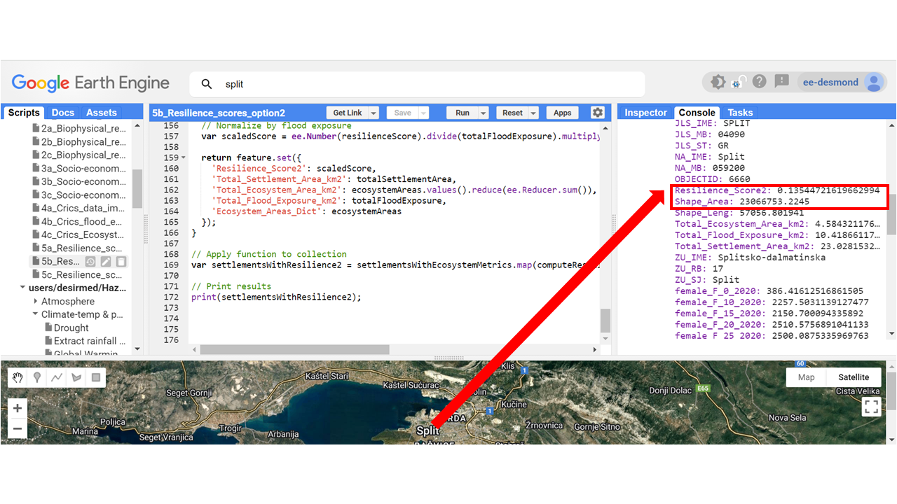
Resilience Score Option 2

This method calculates a resilience score based on ecosystem contribution and hazard exposure. It integrates ecosystem services and flood risk exposure to estimate resilience levels.

Methodology

The resilience score is computed using the following formula:

        Resilience Score = ( Σ (Ecosystem_Area / Total_Settlement_Area × Weight) / Flood_Exposure_Area ) × 10
        

Where:

• Ecosystem_Area: Area covered by a specific ecosystem class.
• Total_Settlement_Area: Total area of the settlement.
• Weight: Importance of the ecosystem in providing resilience.
• Flood_Exposure_Area: Total flood-prone area (sum of high, medium, and low probability flood areas).

    function computeResilienceScore(feature) {
      var weightsDict = ee.Dictionary({
        21100: 0.25,  22100: 0.3,  23100: 0.25,  31100: 0.86,  32100: 0.7,
        33100: 0.84,  42100: 0.75,  42200: 0.65,  51000: 0.65,  71100: 0.95,
        71220: 1, 72100: 0.9,  81100: 0.95, 82100: 0.95
      });
    
      var ecosystemAreas = ee.Dictionary(feature.get('Ecosystem_Class_Areas'));
      var totalSettlementArea = ee.Number(feature.geometry().area().divide(1e6)); // Convert to km²
      var validTotalArea = totalSettlementArea.max(1e-6); // Avoid division by zero
    
      var floodHP = ee.Number(feature.get('Flood_HP_Area_km2'));
      var floodMP = ee.Number(feature.get('Flood_MP_Area_km2'));
      var floodLP = ee.Number(feature.get('Flood_LP_Area_km2'));
      var totalFloodExposure = floodHP.add(floodMP).add(floodLP).max(1e-6);
    
      var resilienceScore = ecosystemAreas.map(function(classValue, area) {
        var classNumber = ee.Number.parse(ee.String(classValue));
        var weight = weightsDict.get(classNumber, 0);
        return ee.Number(area).divide(validTotalArea).multiply(ee.Number(weight));
      }).values().reduce(ee.Reducer.sum());
    
      var scaledScore = ee.Number(resilienceScore).divide(totalFloodExposure).multiply(10);
    
      return feature.set({
        'Resilience_Score2': scaledScore,
        'Total_Settlement_Area_km2': totalSettlementArea,
        'Total_Ecosystem_Area_km2': ecosystemAreas.values().reduce(ee.Reducer.sum()),
        'Total_Flood_Exposure_km2': totalFloodExposure,
        'Ecosystem_Areas_Dict': ecosystemAreas
      });
    }
    
    // Apply function to feature collection
    var settlementsWithResilience2 = settlementsWithEcosystemMetrics.map(computeResilienceScore);
    
    // Print results
    print(settlementsWithResilience2.limit(5));
        

Explanation of the Code

• weightsDict: Defines the resilience weight for different ecosystem classes.
• ecosystemAreas: Retrieves the dictionary of ecosystem areas from the feature.
• totalSettlementArea: Computes the total settlement area in square kilometers.
• totalFloodExposure: Sums up flood-prone areas to quantify risk exposure.
• ecosystemAreas.map(): Loops through each ecosystem class and calculates its contribution.
• resilienceScore: Aggregates all ecosystem contributions based on their weight.
• scaledScore: Normalizes the resilience score by dividing it by total flood exposure.

Why This is an Enhancement Over Option 1

Option 1 simply took the ratio of total ecosystem area to flood exposure area, which does not account for ecosystem diversity or weighting.

This enhanced option improves upon that by:

• Using ecosystem-specific weights to capture their individual contributions.
• Normalizing the resilience score based on the settlement area and flood exposure.
• Making resilience a function of both hazard exposure and ecosystem services.

If you consider both **ecosystem weight and flood exposure**, this option provides a more comprehensive understanding of resilience dynamics.

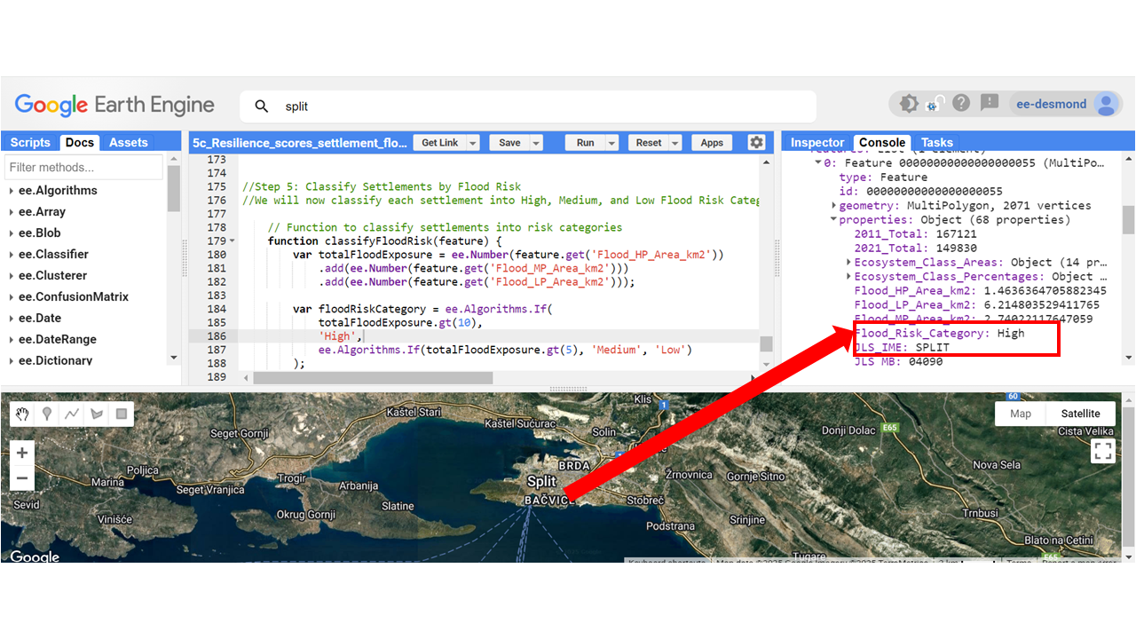
Step 5: Classify Settlements by Flood Risk

We will now classify each settlement into High, Medium, and Low Flood Risk Categories based on its total flood exposure.

    // Function to classify settlements into risk categories
    function classifyFloodRisk(feature) {
        var totalFloodExposure = ee.Number(feature.get('Flood_HP_Area_km2'))
            .add(ee.Number(feature.get('Flood_MP_Area_km2')))
            .add(ee.Number(feature.get('Flood_LP_Area_km2')));
    
        var floodRiskCategory = ee.Algorithms.If(
            totalFloodExposure.gt(10),
            'High',
            ee.Algorithms.If(totalFloodExposure.gt(5), 'Medium', 'Low')
        );
    
        return feature.set('Flood_Risk_Category', floodRiskCategory);
    }
    
    var settlementsWithFloodRisk = settlementsWithResilience.map(classifyFloodRisk);
    

• Settlements with more than 10 km² of flood exposure are classified as High Risk.
• Settlements between 5–10 km² of flood exposure are classified as Medium Risk.
• Settlements below 5 km² of flood exposure are classified as Low Risk.

Impact Chain Assessment

This guide walks you through the **three-step process** of impact assessment using Google Earth Engine (GEE). We'll explore how to analyze **Points of Interest (POIs), Governance & Environmental Data, and Flood Impact Assessment**.

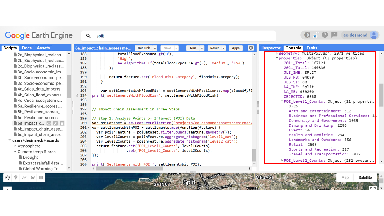
Step 1: Analyze Points of Interest (POI) Data

We begin by integrating **POI data** into settlement areas to understand the socio-economic infrastructure available in different locations.

// Load POI dataset
var poiDataset = ee.FeatureCollection('projects/ee-desmond/assets/desirmed/PointOfinterest');

// Process settlements with POI information
var settlementsWithPOI = settlements.map(function(feature) {
    var poiInFeature = poiDataset.filterBounds(feature.geometry());
    var level1Counts = poiInFeature.aggregate_histogram('level1_cat');
    var level2Counts = poiInFeature.aggregate_histogram('level2_cat');
    return feature.set('POI_Level1_Counts', level1Counts)
                  .set('POI_Level2_Counts', level2Counts);
});

• poiDataset.filterBounds(feature.geometry()): Retrieves all **POIs** that fall within the boundaries of each settlement.
• aggregate_histogram('level1_cat'): Counts the **number of POIs** in each **Level 1 category**.
• aggregate_histogram('level2_cat'): Counts the **number of POIs** in each **Level 2 category**.

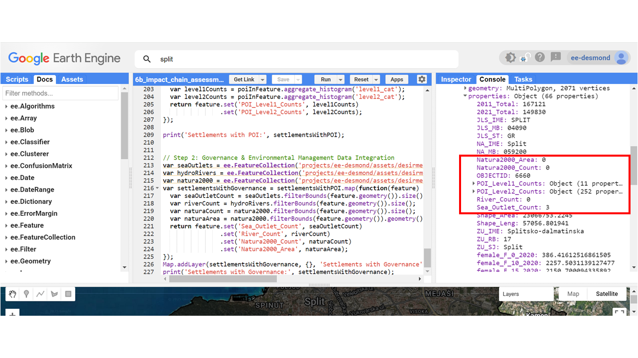
Step 2: Governance & Environmental Management Data Integration

We integrate additional **governance and environmental datasets** such as **sea outlets, hydro-rivers, and protected areas (Natura2000)**.

// Load environmental datasets
var seaOutlets = ee.FeatureCollection('projects/ee-desmond/assets/desirmed/seaoutletclip');
var hydroRivers = ee.FeatureCollection('projects/ee-desmond/assets/desirmed/HydroRIVERS_v10_eu_Clip');
var natura2000 = ee.FeatureCollection('projects/ee-desmond/assets/desirmed/naturaclip2000');

// Process settlements with governance data
var settlementsWithGovernance = settlementsWithPOI.map(function(feature) {
    var seaOutletCount = seaOutlets.filterBounds(feature.geometry()).size();
    var riverCount = hydroRivers.filterBounds(feature.geometry()).size();
    var naturaCount = natura2000.filterBounds(feature.geometry()).size();
    var naturaArea = natura2000.filterBounds(feature.geometry()).geometry().area().divide(1e6);
    return feature.set('Sea_Outlet_Count', seaOutletCount)
                  .set('River_Count', riverCount)
                  .set('Natura2000_Count', naturaCount)
                  .set('Natura2000_Area', naturaArea);
});

• filterBounds(feature.geometry()): Selects governance-related features **inside each settlement**.
• size(): Counts the **total number** of features (e.g., sea outlets, rivers, Natura2000 sites).
• geometry().area().divide(1e6): Converts the area of protected sites from **square meters to square kilometers**.

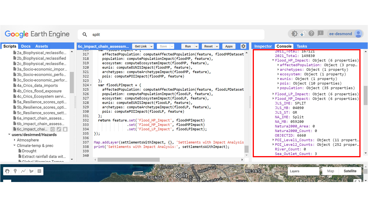
Step 3: Impact Assessment (Flood Exposure, Ecosystem, Archetypes, EUNIS, Population, Age, and Sex)

Now we assess the impact of **flood hazards** on different settlements, integrating **demographics, ecosystems, and land classifications**.

// Load flood datasets
      // Step 3: Impact Assessment (Flood Exposure, Ecosystem, Archetypes, Eunis, Population, age and sex)
      var floodHPDataset = ee.FeatureCollection("projects/ee-desmond/assets/desirmed/floods_HP_2019");
      var floodMPDataset = ee.FeatureCollection("projects/ee-desmond/assets/desirmed/floods_MP_2019");
      var floodLPDataset = ee.FeatureCollection("projects/ee-desmond/assets/desirmed/floods_LP_2019");
      var worldPop = ee.ImageCollection('WorldPop/GP/100m/pop_age_sex');
      
      // General population data for multiple years
      function computeAffectedPopulation(feature, floodDataset, years) {
        var impactedFlood = floodDataset.filterBounds(feature.geometry());
        var popImpacts = {};
        years.forEach(function (year) {
          var yearKey = 'pop_' + year;
          var totalPopulation = feature.get(yearKey);
          var affectedArea = impactedFlood.geometry().area();
          var settlementArea = feature.geometry().area();
          var proportionAffected = ee.Number(affectedArea).divide(settlementArea);
          var affectedPopulation = ee.Number(totalPopulation).multiply(proportionAffected);
          popImpacts[year] = affectedPopulation;
        });
        return ee.Dictionary(popImpacts);
      }
      
      // Define demographic bands
      var demographicBands = worldPop.select([
        'population', 'M_0', 'M_5', 'M_10', 'M_15', 'M_20', 'M_25', 'M_30', 'M_35', 'M_40',
        'M_45', 'M_50', 'M_55', 'M_60', 'M_65', 'M_70', 'M_75', 'M_80',
        'F_0', 'F_5', 'F_10', 'F_15', 'F_20', 'F_25', 'F_30', 'F_35', 'F_40', 'F_45',
        'F_50', 'F_55', 'F_60', 'F_65', 'F_70', 'F_75', 'F_80'
      ]);
      
      // Define computation functions
      function computePopulationImpact(flood, feature) {
        return demographicBands.mean().reduceRegion({
          reducer: ee.Reducer.sum(),
          geometry: flood.geometry().intersection(feature.geometry(), ee.ErrorMargin(1)),
          scale: 100,
          maxPixels: 1e13
        });
      }
      
      function computeEcosystemImpact(flood, feature) {
        return ecosystemServices.reduceRegion({
          reducer: ee.Reducer.frequencyHistogram(),
          geometry: flood.geometry().intersection(feature.geometry(), ee.ErrorMargin(1)),
          scale: 30,
          maxPixels: 1e13
        });
      }
      
      function computeEUNISImpact(flood, feature) {
        return eunis.reduceRegion({
          reducer: ee.Reducer.frequencyHistogram(),
          geometry: flood.geometry().intersection(feature.geometry(), ee.ErrorMargin(1)),
          scale: 30,
          maxPixels: 1e13
        });
      }
      
      function computeArchetypeImpact(flood, feature) {
        return archetypes.reduceRegion({
          reducer: ee.Reducer.frequencyHistogram(),
          geometry: flood.geometry().intersection(feature.geometry(), ee.ErrorMargin(1)),
          scale: 30,
          maxPixels: 1e13
        });
      }
      
      function computePOIImpact(flood, feature) {
        var poiInFlood = poiDataset.filterBounds(flood.geometry().intersection(feature.geometry(), ee.ErrorMargin(1)));
        return poiInFlood.aggregate_histogram('level1_cat');
      }
      
      var years = [2020, 2025, 2030];
      var settlementsWithImpact = settlementsWithGovernance.map(function (feature) {
        var floodHP = floodHPDataset.filterBounds(feature.geometry());
        var floodMP = floodMPDataset.filterBounds(feature.geometry());
        var floodLP = floodLPDataset.filterBounds(feature.geometry());
      
        var floodHPImpact = {
          affectedPopulation: computeAffectedPopulation(feature, floodHPDataset, years),
          population: computePopulationImpact(floodHP, feature),
          ecosystem: computeEcosystemImpact(floodHP, feature),
          eunis: computeEUNISImpact(floodHP, feature),
          archetypes: computeArchetypeImpact(floodHP, feature),
          pois: computePOIImpact(floodHP, feature)
        };
        var floodMPImpact = {
          affectedPopulation: computeAffectedPopulation(feature, floodMPDataset, years),
          population: computePopulationImpact(floodMP, feature),
          ecosystem: computeEcosystemImpact(floodMP, feature),
          eunis: computeEUNISImpact(floodMP, feature),
          archetypes: computeArchetypeImpact(floodMP, feature),
          pois: computePOIImpact(floodMP, feature)
        };
        var floodLPImpact = {
          affectedPopulation: computeAffectedPopulation(feature, floodLPDataset, years),
          population: computePopulationImpact(floodLP, feature),
          ecosystem: computeEcosystemImpact(floodLP, feature),
          eunis: computeEUNISImpact(floodLP, feature),
          archetypes: computeArchetypeImpact(floodLP, feature),
          pois: computePOIImpact(floodLP, feature)
        };
        return feature.set('Flood_HP_Impact', floodHPImpact)
                      .set('Flood_MP_Impact', floodMPImpact)
                      .set('Flood_LP_Impact', floodLPImpact);
      });
      
      Map.addLayer(settlementsWithImpact, {}, 'Settlements with Impact Analysis');
      print('Settlements with Impact Analysis:', settlementsWithImpact);
    

• floodDataset.filterBounds(feature.geometry()): Extracts **flood-affected areas** within each settlement.
• affectedArea = impactedFlood.geometry().area(): Computes the **area of affected regions**.
• settlementArea = feature.geometry().area(): Measures the **total area of the settlement**.
• proportionAffected = affectedArea.divide(settlementArea): Determines **how much of the settlement is affected**.
• affectedPopulation = totalPopulation.multiply(proportionAffected): Estimates **the number of affected people**.

We have integrated **spatial, demographic, and environmental data** to assess flood risk and how it relates to the various landscape characters.

We have now:

• Loaded and analyzed flood exposure across settlements.
• Computed the role of ecosystem services in buffering flood risks.
• Assigned resilience scores to settlements.
• Classified settlements into High, Medium, and Low Risk zones per the 3 domains.
• Visualized the results

You can explore the engine app with vSisualised layers here